
What a chute has to do
It sounds simple: take the material coming off one belt and put it on the next. In practice there are four jobs, and each has its own way of failing.
- Receive the material at head-pulley speed, without it slamming into the front wall and bouncing back.
- Redirect the flow, often by 90 degrees, without scattering it.
- Control the velocity of the drop, because too much energy on arrival turns into wear, particle breakage and dust.
- Deliver it centred on the receiving belt, already in its direction and close to its speed, so as not to mistrack the belt or tear its cover.
Whatever goes wrong is always one of those four. Wear on the plate where the stream hits. Blockage when wet material sticks in a corner. Spillage when the load arrives off-centre. A punctured belt when large rocks fall from height onto the carcass. And the worst part is that nearly all of it only shows up after installation, because a chute is a closed box where nobody sees what happens.
That "nobody sees" is exactly what simulation fixes.
Case 1: the straight-drop chute
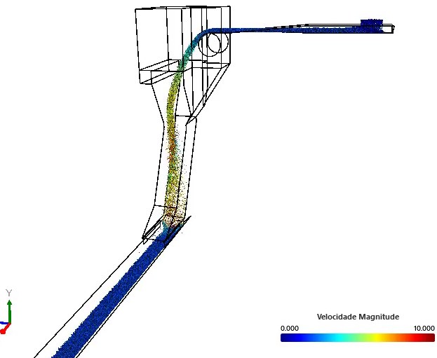
The first case is the most common design there is: a box that receives the stream from the upper head pulley and lets it fall onto the lower belt, which runs perpendicular. The geometry came straight from a STEP file of the real equipment, with both belts modelled as moving surfaces.
Three things stand out in the animation:
- The material accelerates throughout the fall. There is nothing in the way to slow it, so it arrives at the bottom in the hot end of the scale.
- The stream arrives concentrated in a narrow band of the receiving belt. That is where the cover will wear, and where a large rock can puncture the carcass.
- The arrival direction is vertical while the belt runs horizontal. Every bit of horizontal velocity the material needs, it has to gain through friction with the belt, and that is more wear.
The case was run with two materials, a generic granular and pellets, precisely to see whether the answer changes with the type of load. The chute geometry is the same; what changes is the calibration.
Case 2: the cascade chute
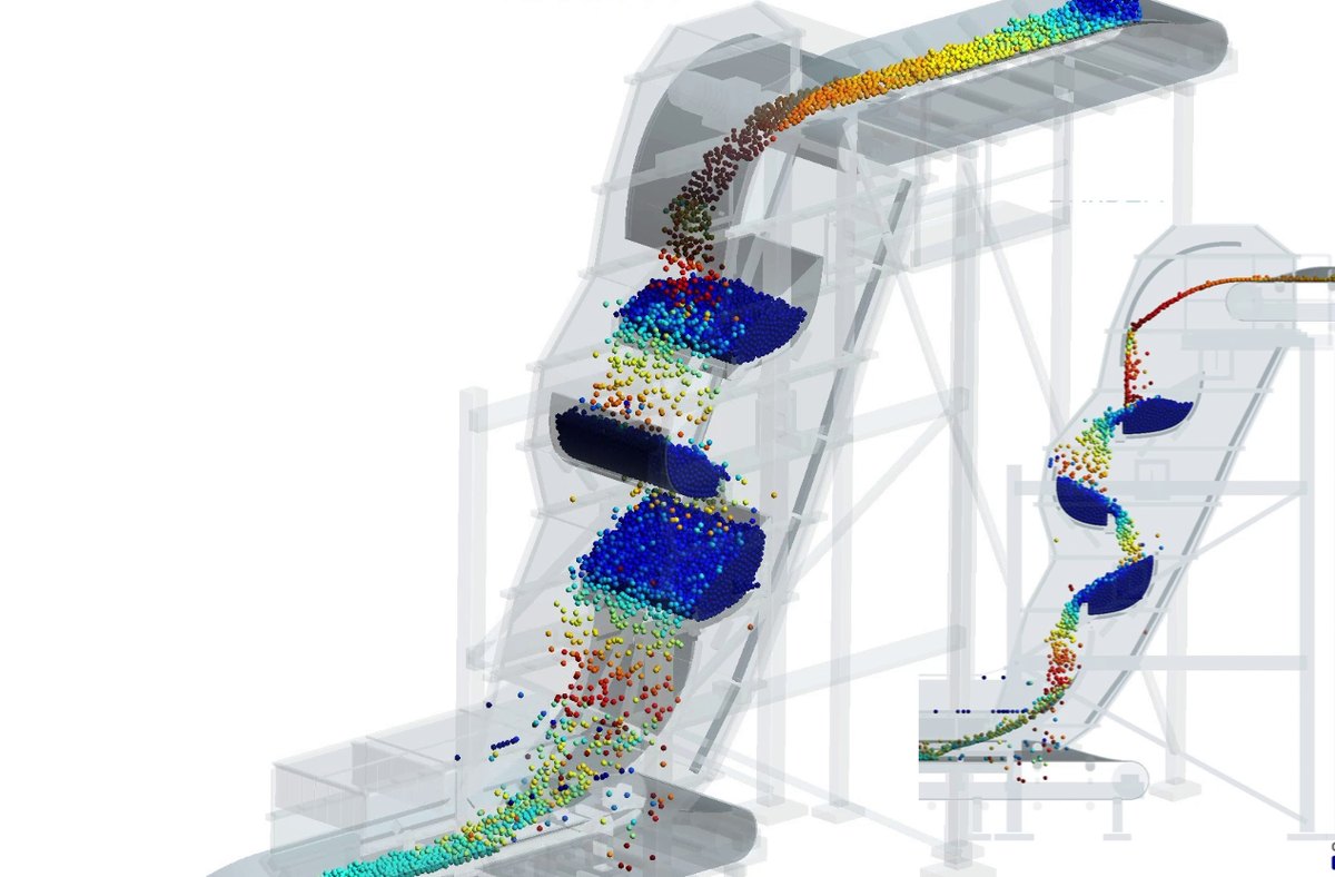
The second case solves the velocity problem in an old and effective way: instead of letting the material fall in one go, it places a series of curved deflectors in the path that break the drop into stages. Each deflector holds a bed of stationary material, and incoming material slides over that bed, not over the steel.
The close-up on the deflectors is what explains the concept best:
The idea is that wear happens material against material, which is free, rather than material against steel, which costs plate. And that each stage gives back part of the energy the drop has built up, so the material reaches the lower belt ready to land rather than strike.
What the cascade numbers say
Here case 2 has the edge, because it ran for 50 seconds with every output switched on. The data below is BrixDEM output, unadjusted.
Throughput: the chute has to "prime" before it works
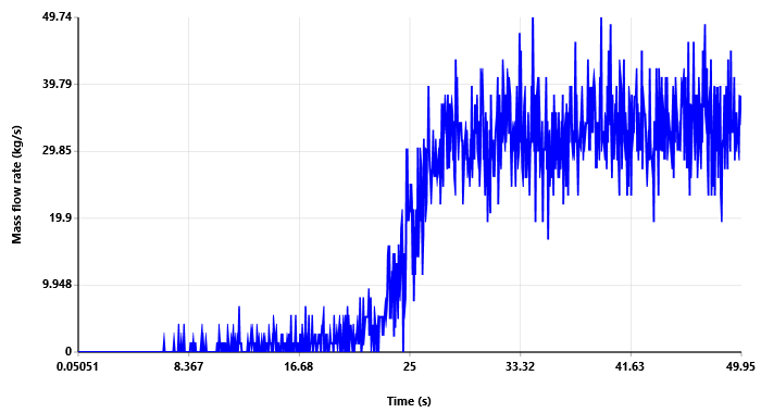
This chart surprises anyone who has never simulated a cascade chute. The feed is constant from the start, yet the outlet sits near zero for 16 seconds, climbs slowly until 24, and only then jumps to the steady 33 kg/s. The reason is that the four deflectors have to build their dead beds before letting material through. Until then, the chute is storing material, not transferring it.
At steady state there are about 880 kg inside the system across beds, belts and material in flight. That matters at two moments: on start-up, because the lower belt is slow to receive load; and on shutdown, because all that material keeps coming down after the feed stops.
Velocity: nearly everything is standing still
The maximum velocity in the system is around 6.4 m/s, reached by material in free fall between one deflector and the next. The mean velocity, though, is 0.63 m/s. The gap between those two numbers is the very definition of a cascade: most of the mass sits in the dead beds without moving, and only a small fraction is in transit at any instant.
Wear: where the plate will open up
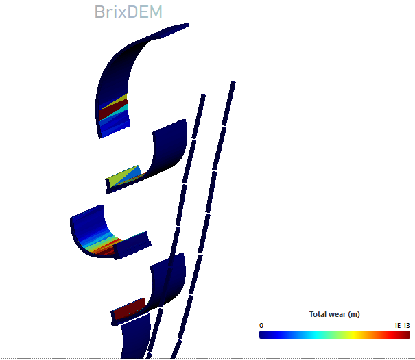
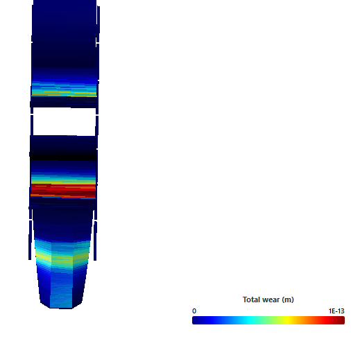
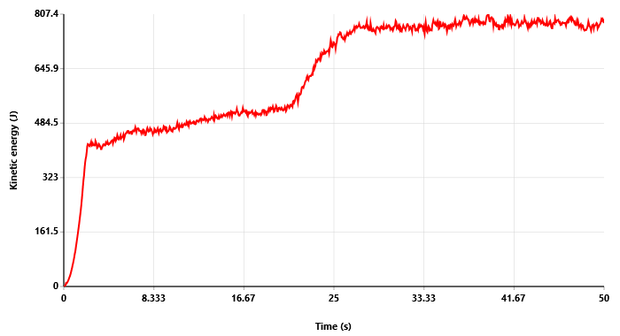
The map answers the maintenance question before the plate exists. Wear is not uniform: it concentrates in a narrow band on the impact face of each deflector, exactly where the stream from above meets the bed. Sides, bottom and casing barely suffer. That says where to put liners, how much plate to keep in stock and which deflector will need replacing first.
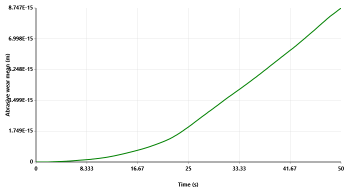
The accumulated wear curve has the same knee as the throughput chart, and that is no coincidence. While the chute is priming there is little material in transit and little friction. Once it reaches steady state, wear grows in a straight line, and the slope of that line is what gets extrapolated to estimate service life in operating hours.
One against the other
| Straight drop | Cascade | |
|---|---|---|
| Arrival velocity | high; accelerates the whole drop | cut at each deflector |
| Where it wears | receiving belt and impact plate | deflector impact faces, material on material |
| Height needed | less | more; each stage needs room |
| Start-up and shutdown | immediate response | slow to prime; keeps discharging after stop |
| Material held | almost none | hundreds of kilos in the dead beds |
| Risk with wet or cohesive material | low | high; a dead bed can become a stuck bed |
| Design complexity | low | medium; deflector position and curvature matter |
Neither one is "the right one". The straight drop is simple, cheap and responds instantly, at the cost of punishing the receiving belt. The cascade protects belt and plate, at the cost of height, held-up material and a serious risk with sticky material. The choice depends on the material, the height available and what it costs to stop the line to replace belt cover.
What simulation lets you decide
- Where to line. The wear map shows the impact bands. Liner anywhere else is money thrown away.
- How many deflectors, and where. Moving a deflector a few centimetres changes where the stream hits the next one. That is tested in minutes in simulation and in weeks on site.
- Whether the lower belt will suffer. Arrival velocity and landing point say whether the material lands or strikes, and whether it arrives centred.
- How much material is held up. For sizing start-up, shutdown and what happens in an emergency.
- Whether it will block. Run the same chute with the material calibrated wet. If a dead bed stops spilling over, the design has a problem that would only show up on the first rainy day.
Simulate your chute before cutting plate
Import the CAD (STEP, IGES or STL), set the belts in motion and read throughput, arrival velocity and the wear map before the part exists.