
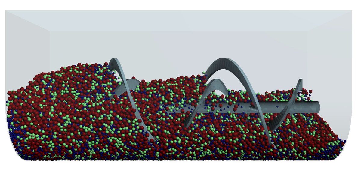
The case
The equipment is a ribbon mixer: a U-shaped trough with a double-helix rotor that pushes material outwards along the outer ribbon and brings it back through the centre. It is the most common mixer for dry solids, from animal feed to mortar.
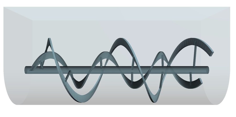
The charge is not uniform. Particles range from 10 to 20 mm in radius and are split into three materials, tracked separately across 20 seconds of simulation. That spread of sizes is what makes the case interesting, and it is also the reality of nearly every industrial powder or granular product.
How "mixing" is measured
Watching the animation does not settle it. The bed looks well mixed from start to finish, and nobody can see a few percent of difference in uniformity. So DEM divides the volume into sampling regions and computes, at every instant, how much composition varies from one region to the next.
Two metrics do the job:
| Lacey index | Coefficient of variation (CV) | |
|---|---|---|
| What it is | measured variance against the two theoretical extremes | standard deviation divided by mean concentration |
| Scale | 0 = fully segregated, 1 = perfectly random | 0 = uniform, grows with no upper bound |
| Better when | closer to 1 | closer to 0 |
| Strength | normalised, so cases can be compared | direct and easy to explain |
It is worth using both. The Lacey index is bounded between 0 and 1, which helps when comparing different equipment. CV is more intuitive for anyone used to quality control, because it speaks the same language as a sampling report.
What the simulation showed
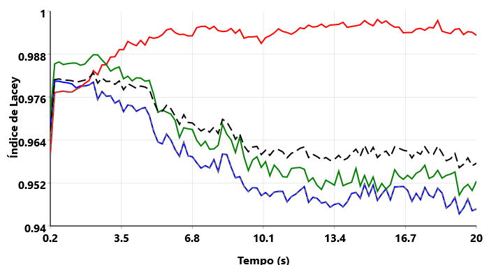
Reading the chart:
- Everything rises in the first few seconds. The rotor grabs the freshly inserted charge and spreads it quickly, and every fraction reaches roughly 0.98.
- One fraction keeps improving and settles around 0.995, essentially random.
- The other two go the other way. Between 5 and 10 seconds they drop from about 0.977 to the 0.948–0.952 range, and stay there to the end.
- The global average (dashed) falls from 0.980 to about 0.957.
Why it degrades: size segregation
The culprit is the size difference. When a granular bed is agitated, momentary voids open up between the large particles. A small particle fits into those voids and slips downwards; a large one does not fit and stays put. Repeat that thousands of times and the result is systematic: fines go down, coarse goes up.
The technical name is percolation, and it is the same effect that drives the larger nuts to the top of the tin. In a ribbon mixer it is especially stubborn, because the circulation the rotor imposes is exactly what keeps the bed moving and feeds the percolation. The equipment mixes and segregates at the same time, with the two mechanisms competing.
Early on, mixing wins, because the charge arrives disorganised and there is plenty to homogenise. Once the material is spread out there is little mixing left to do, and segregation takes over. The crossover between the two is exactly the knee in the chart.
The coefficient of variation tells the same story
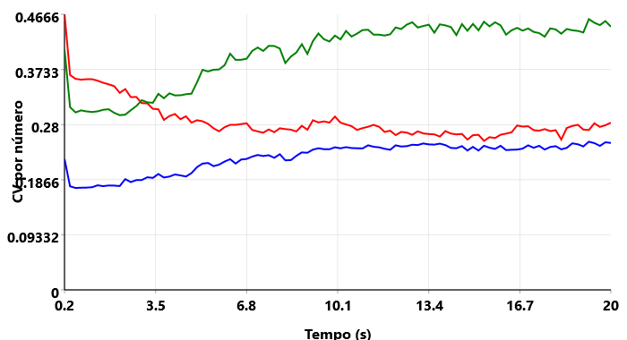
One fraction goes from 0.30 to 0.45, meaning it ends up fifty percent more dispersed than it started. Another does the reverse, falling from 0.46 to 0.28. The third rises mildly, from 0.19 to 0.25.
Two independent metrics pointing the same way is what gives the diagnosis its confidence. Had only the Lacey index dropped, it would be fair to suspect the size of the sampling regions instead.
What it costs to keep mixing
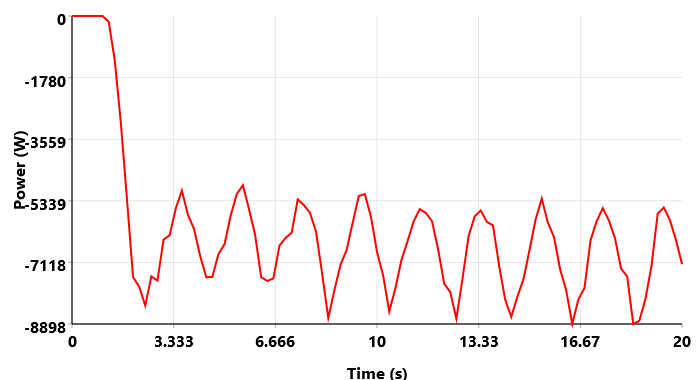
After start-up, power settles into an oscillation between roughly 5 and 9 kW. The oscillation is regular and follows the ribbon sweeping through the charge: on each turn the rotor meets more material on one side, torque climbs, then eases off.
Put that together with the previous chart and the cost shows up: the 15 seconds after the optimum consumed something on the order of 100 kJ and delivered a worse mixture. On equipment running batches all day, that is money and quality leaking in both directions.
Applying this to your own equipment
The procedure is short:
- Calibrate the material first. Without representative friction and cohesion, the segregation rate comes out wrong and so does the optimal time. The calibration guide covers it.
- Use the real size distribution, not a mean diameter. Size segregation is the effect under study; simulating everything at one size erases exactly what you want to see.
- Track each fraction separately, not just the average. It was a single fraction that exposed the problem here; the average alone hides it.
- Run longer than you intend to operate. The knee in the curve only appears if the simulation goes past it.
- Read Lacey and CV together. Agreement between the two is a sign the result is not a sampling artefact.
The takeaway
Mixing quality is not something you assess by looking. In this case the bed appeared perfectly homogeneous throughout all 20 seconds, while two of the three fractions were slowly pulling apart. It had to be measured to be seen, and measuring is cheap when it happens in simulation rather than in the plant.
The practical question this kind of study answers is not "does my mixer mix?" but "when should I stop?". The answer is usually sooner than expected.
Measure mixing in your own equipment
BrixDEM computes the Lacey index, coefficient of variation, power and energy while the simulation runs. Build your mixer and find the optimal time.