
What a screw conveyor is
It is a helical flight rotating inside a trough or tube. With every turn, the material trapped between the flights is pushed one pitch forward. Simple to build, enclosed (so it does not spread dust) and compact, it shows up in cement plants, grain silos, feed mills, waste treatment, food, chemicals and mining.
In practice the problems are almost always the same: fill level different from the assumption, throughput below expectation, pulsating discharge, wear concentrated on the flight and the trough, and an undersized motor that stalls at start-up or on load peaks.
Why simulate a screw conveyor with DEM
Classic sizing methods compute throughput and power from empirical fill and material factors. They work well for catalogue geometries and products, but they say very little about the specific material you are going to convey.
The Discrete Element Method takes a different route: it simulates every particle and the contact forces between them and with the equipment. That lets you see the actual fill level, how the load is distributed along the length, how much the material slips, where wear will start and how much power the shaft really demands.
The simulated case
The setup is as representative as it gets: a hopper feeds by gravity into a horizontal screw, which conveys the material to the discharge at the opposite end. The run covers 50 seconds of simulated time, and the material travels about 4 metres along the axis.
What has to be defined in the software
- Geometry: the trough and the helical flight, imported from CAD or drawn in the built-in modeler.
- Motion: rotation of the flight about its own axis, in rpm.
- Material: density, contact stiffness, coefficient of restitution, sliding friction and rolling friction, all calibrated for the real product.
- Feed: the hopper as a particle source, to reproduce the gravity inlet.
- Measurement: a region at the discharge to account for the mass and the number of particles leaving.
Why the material advances instead of spinning along
One detail explains how the whole machine works: the material does not rotate with the flight. If it did, it would simply spin in circles and there would be no transport at all. It is the friction against the trough wall that holds the material back and converts shaft rotation into travel along the tube.
That is why particle-wall friction is such a sensitive parameter in a screw conveyor: calibrate it wrong and the simulation conveys too much or too little. Near the end of the run the screw is full along its whole length and discharges continuously.
Result 1: instantaneous throughput at the discharge
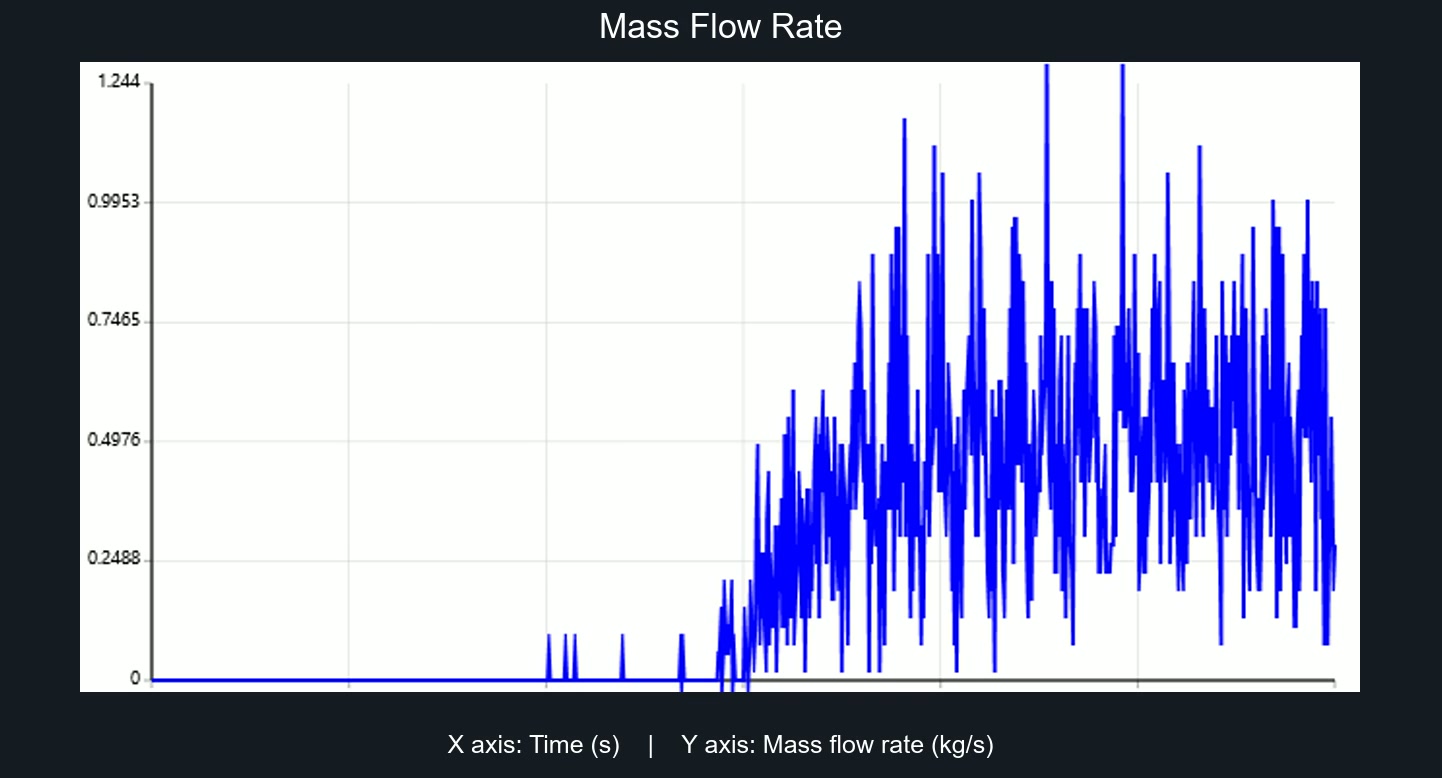
The reading is straightforward: nothing leaves the screw in the first seconds. The first grains cross the discharge at around 17 s (those isolated spikes), and only from 25 s onwards is the flow truly established, oscillating between roughly 0.25 and 1.24 kg/s.
Why does it oscillate so much? Because the discharge of a screw conveyor is not continuous. Every pitch of the flight pushes a packet of material out, and we are counting discrete particles crossing a plane. This pulsation is real, not numerical noise, and it is exactly why the instantaneous value is the worst possible basis for sizing anything.
The solver also records the same throughput in particles per second, with an identically shaped curve. That gives you a quick sanity check: dividing the average mass flow rate by the average particle rate gives about 2.6 g per particle. If that value does not match the density and diameter you defined, something is wrong in the setup.
Result 2: cumulative mass, the most reliable result
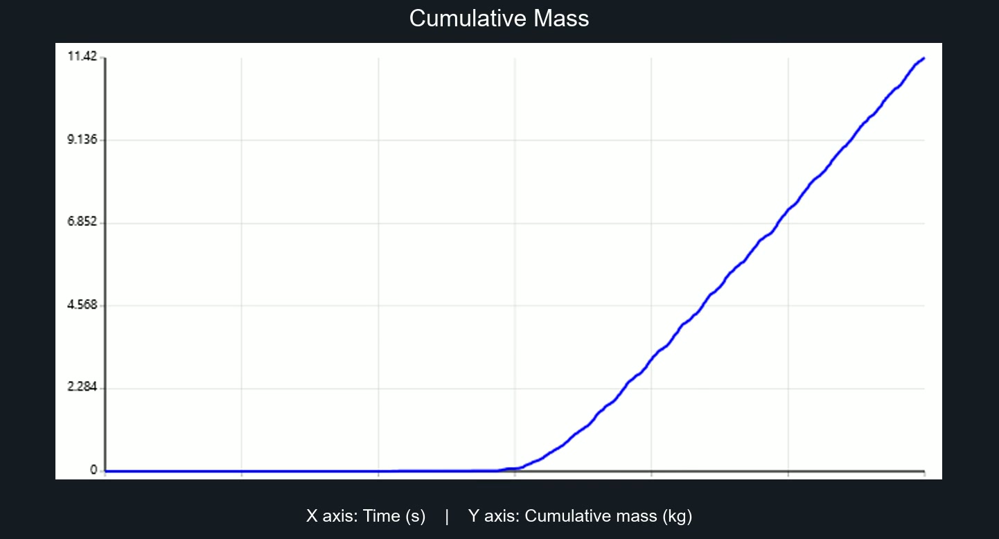
This is the curve you should use. Because it is the integral of the flow rate, all the pulsation noise disappears and what remains is a clean straight line. After 50 s, 11.42 kg had been discharged, and the curve starts rising at around 25 s.
The design throughput comes from the slope of the straight segment:
Keep this rule in mind: in any conveying equipment, reliable throughput comes from the slope of the cumulative mass during steady state, never from averaging a spiky instantaneous signal.
Result 3: mechanical power
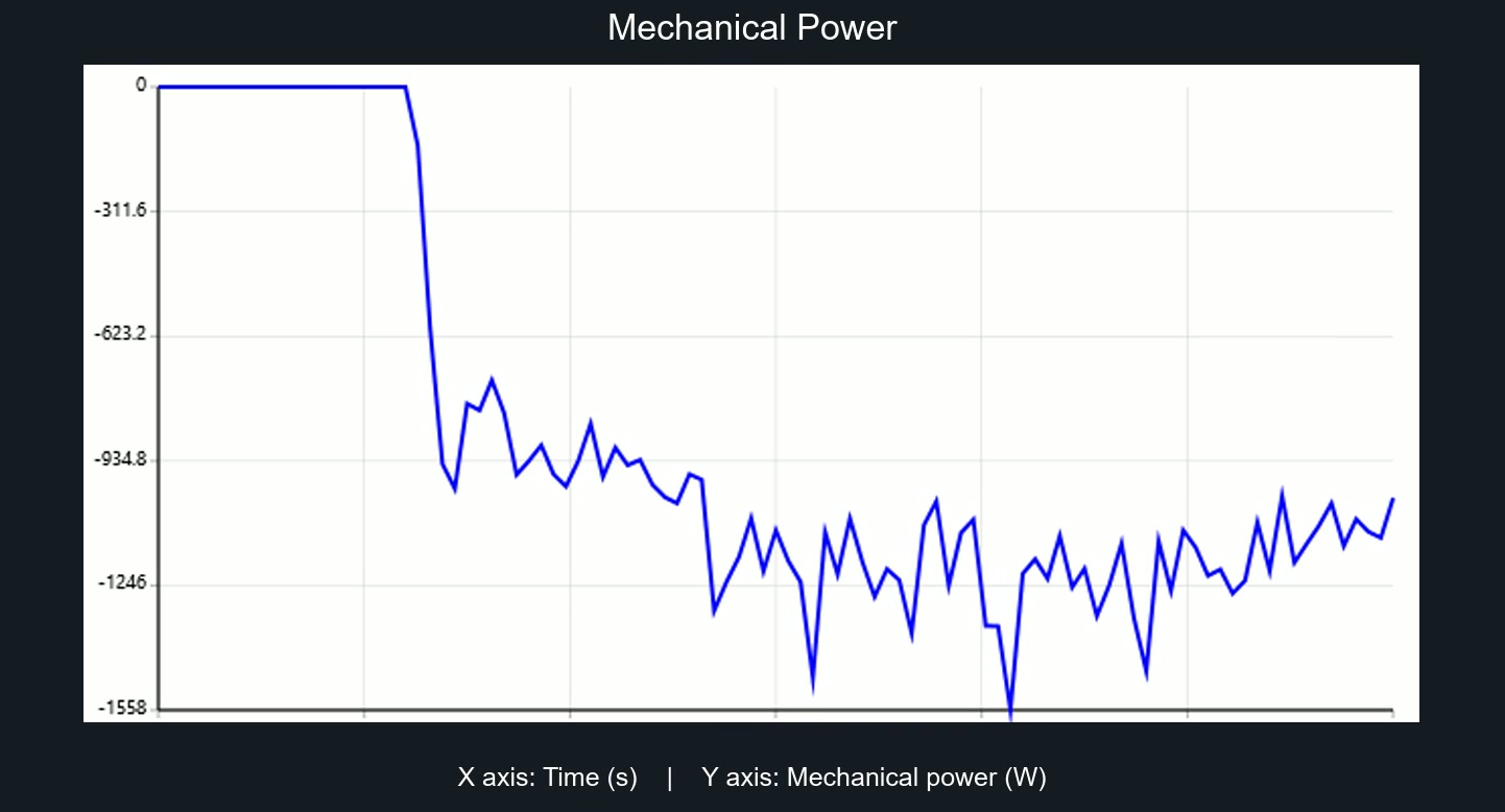
Power tells the story of how the screw fills up. It stays at zero until about 10 s, while the flight is still turning essentially empty. When material comes in, it jumps straight to nearly 900 W and then settles between 1.1 and 1.3 kW, with peaks up to 1.56 kW.
That gradual increase has a simple physical explanation: the screw becomes full along its entire length, so more and more material is being dragged at the same time. And the oscillation about the mean is the same pulsation we saw in the flow rate, now felt as torque variation.
Here is the classic design mistake: choosing the motor from the average. A drive sized for 1.2 kW will struggle at the 1.56 kW peaks, which are about 30% higher. Size from the peak and still add the start-up margin, when the screw may be full and stopped.
With throughput and power together you can compute the specific energy, which is excellent for comparing design alternatives: about 1.2 kW ÷ 1.6 t/h ≈ 0.73 kWh per tonne conveyed.
The four lessons from this case
- Discard the transient. Here the first 25 s are filling, not operation. Including them in the average underestimates throughput.
- Take throughput from the cumulative mass. The slope of the straight segment is the design figure.
- Size the motor from the peak. The average misleads, because granular material works in pulses.
- Run the consistency check. Mass per particle, fill level and residence time all have to make physical sense.
What else this model can deliver
- Wear: abrasion maps show where the flight and the trough will wear first, typically at the outer edge of the flights and in the inlet region.
- Rotation speed: increasing rpm does not always increase throughput. Above a certain speed the material starts being thrown instead of pushed.
- Inclination: inclined screws lose efficiency quickly, and DEM quantifies that loss.
- Backflow: the clearance between flight and trough creates return flow, which shows up directly in the simulated throughput.
- Shaft torque: the basis for the mechanical sizing of the auger and its bearings.
How to reproduce it in BrixDEM
The recipe is short: draw or import the trough and the flight, apply rotation to the flight, calibrate the material with the angle of repose and inclined plane tests, place the hopper as a particle source and create the measurement region at the discharge. Then run it and export the throughput, cumulative mass and power curves, exactly like the ones in this article.
Download BrixDEM and build the case following this recipe. If you would rather see the setup first, the video tutorials walk through it step by step on other equipment, and the same logic applies to the screw.
Have a look as well at other simulated equipment, such as mixers, rotary drums, chutes and elevators.
Frequently asked questions
Do I need particles at the real product size?
Not always. It is common DEM practice to work with particles larger than the real ones to keep the computational cost feasible, as long as the parameters are calibrated to reproduce the macroscopic behavior of the material, such as the angle of repose.
Why does the simulated throughput differ from the manufacturer's table?
Because the table assumes a typical fill factor and a standard material. The simulation uses the fill level that actually occurs with your geometry, rotation and material. A discrepancy does not mean an error, it means the real fill level is worth investigating.
Can I simulate an inclined or vertical screw?
Yes. You only have to change the orientation of the geometry and the direction of gravity relative to the axis. These are precisely the cases where empirical sizing loses accuracy and DEM helps the most.
How much simulated time is needed?
Enough to get through the transient and still have a usable steady segment. In this case, 50 s gave 25 s of established regime, which is plenty for a reliable slope on the cumulative mass curve.
Simulate your own screw
BrixDEM is free to download and runs on Windows. Build the geometry, define the material and measure throughput and power.