
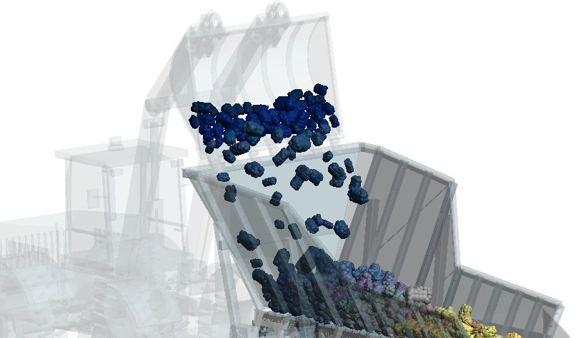
What an apron feeder is and how it works
An apron feeder extracts material from hoppers, bins or stockpiles and delivers it to crushers, conveyors and other process stages. It is used in mining and aggregate processing, particularly where feeding involves large lumps, heavy loads and impacts.
Transport is provided by metal pans driven by chains. The pans support the bed and carry material to discharge. The hopper and sidewalls help guide the load onto the feeder.
Pan speed influences flow, but it is not the only factor. Outlet opening, bed depth, particle size distribution and friction also affect how much material advances. Increasing speed therefore does not guarantee a proportional increase in feed under every condition.
Why simulate an apron feeder with DEM?
Design establishes an operating condition. Simulation helps investigate what happens when actual material meets the geometry: how the load settles, where it is retained and how it reaches downstream equipment.
The Discrete Element Method tracks particle motion and contacts between particles and equipment surfaces. In this example, angular rocks are approximated by clumps, representing a more irregular shape than a single sphere.
- Feed regularity: assess discharge fluctuations at a timescale relevant to the downstream crusher or conveyor.
- Load distribution: observe accumulation and how material occupies the hopper and pans.
- Component loading: track contact forces during loading and transport.
- Alternative designs: test speed, outlet opening, geometry and feeding conditions while keeping other variables controlled.
A useful comparison requires geometry, pan motion, particle size distribution and material contact parameters. Calibration connects these parameters to behaviour observed in physical tests.
What can we extract from the simulation?
The demonstration case
The model starts with material in the hopper and loading bucket. The run follows one dump onto the existing bed and transport by the pans. The data below describe this scenario, rather than an established continuous operation.
| Recorded configuration | Value |
|---|---|
| Physical simulation time | Approximately 20 s |
| Initial population | 16,614 particles |
| Total initial mass | 7.45 t |
| Individual mass range | 0.060 to 10.76 kg |
| Rock representation | Angular clumps |
Mass flow and cumulative discharge
| Discharge result | Value |
|---|---|
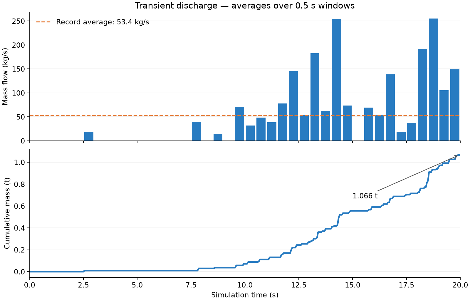
| Cumulative mass by 19.95 s | 1.066 t |
| Average over the full record | 53.4 kg/s — approximately 192 t/h |
| Average recorded rates from 12 to 20 s | 112.0 kg/s — approximately 403 t/h |
The final interval's average is approximately 2.1 times the full-record average. This does not mean capacity doubled: these are different intervals of a transient discharge. Values in t/h are conversions of measured rates, rather than demonstrated sustained capacity.
Cumulative mass helps read this evolution. A steeper curve indicates greater flow over that interval. Assessing continuous operation requires a longer run and a slope that remains consistent over a representative interval.
How discharge fluctuates
At the original resolution of approximately 50 ms, 75% of windows from 10 s onwards record no discharge. The largest window accumulates approximately 79 kg. The chart groups these events into 0.5 s windows to show behaviour at another timescale.
This distinction matters to the process: downstream transport may smooth a short event, while a longer fluctuation may affect feeding. Analysis needs a window suited to the response of downstream equipment.
Feeder contact loads
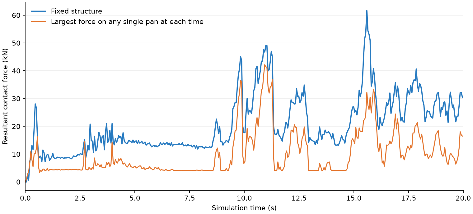
The fixed structure reaches approximately 61.6 kN of resultant contact force. Among the pans, the largest recorded individual peak is 42.2 kN. The histories help identify major loading events and select conditions for structural assessment.
These results represent particle loads. Component weight, inertia, constraints and other loads must also be considered in mechanical design. The pan curve is neither the sum of all pan loads nor the drive traction force.
Regional wear
Alongside curves, DEM provides visualization of predicted wear distribution on surfaces. The map helps investigate regions for protection, liners or geometry changes.
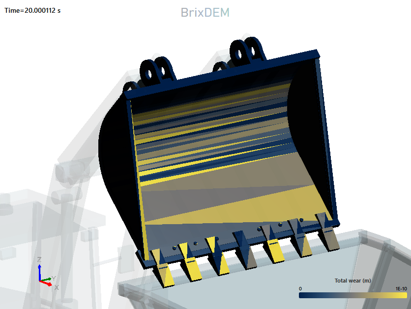
The image demonstrates regional visualization. Feeder wear must be assessed on the feeder's own surfaces. Estimating thickness loss or service life requires model calibration and representative operating conditions.
How to use these results
- Speed and opening: compare flow and fluctuations under the same charge.
- Loading: test feeding frequency and its effect on hopper accumulation.
- Geometry and protection: investigate how surface changes affect flow, forces and predicted wear.
Assess your apron feeder with DEM
Simulate your scenario in BrixDEM or contact us to study your equipment's flow, loading and wear.