
What a silo is (and why the flow is hard to predict)
Silos and hoppers store bulk solids — grain, cement, ore, plastics, pharmaceutical powders — and release them in a controlled way. The typical geometry is a vertical body with a converging hopper bottom that channels the material toward the discharge outlet.
The catch is that a granular material is neither liquid nor solid: it forms force chains, arches over the outlet, flows along preferential paths and separates by size. Hence the classic defects: arching (the material forms an arch and stops flowing), ratholing (only the central core flows, leaving material stuck at the sides), segregation (fines and coarse separate) and pressure peaks at the body–hopper transition that size the structure.
Filling and discharge: the two phases
Every silo simulation goes through two phases. During filling, particles fall and settle to rest — the kinetic energy rises with the impacts and then drops to practically zero, indicating the bed has stabilized. During discharge, the outlet plate is removed and the material flows out by gravity until the silo empties.
It is in the discharge that the design questions live: what is the flow rate? is it mass flow or funnel flow? how long does it take to empty? where are the stagnant zones?
Why simulate silos with DEM
Classic methods (Janssen for pressures, Beverloo for flow rate, Jenike diagrams for the flow type) give good estimates for catalog cases, but say little about your material and your geometry. The Discrete Element Method solves the problem particle by particle: it simulates every grain and every contact, so you see the real filling, the flow pattern, the instantaneous flow rate, the wall forces and exactly where the material gets stuck.
Flow pattern: mass flow vs. funnel flow
The discharge pattern defines the quality of a silo. In mass flow, all the material descends together — first in, first out — which avoids dead zones and reduces segregation. In funnel flow, only a central column flows and the rest stays put, favoring ratholing and stagnant product.
In DEM this is visible by coloring the particles: in the video, coloring by particle ID shows the layers descending in order and deforming into a "V" only inside the hopper — the signature of mass flow. Coloring by velocity magnitude reveals where the material accelerates, always toward the outlet.
Discharge rate
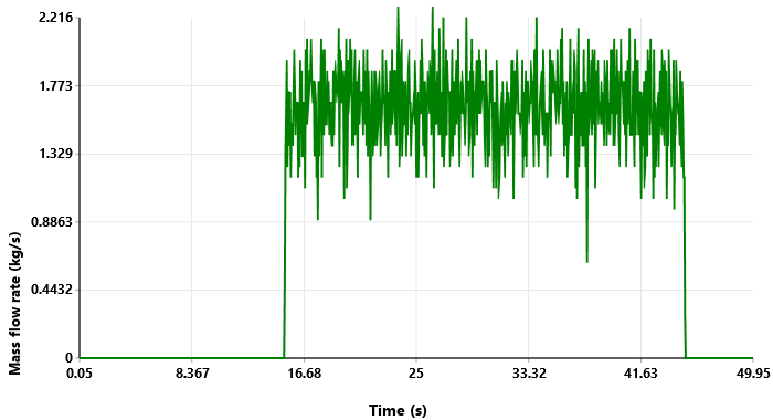
A striking feature of the silo: the discharge rate is constant and independent of the material head above the outlet — the basis of Beverloo's equation. That is why the curve reaches a plateau and stays there. The oscillation around the mean is physical, caused by discrete particles crossing the outlet plane, not numerical noise.
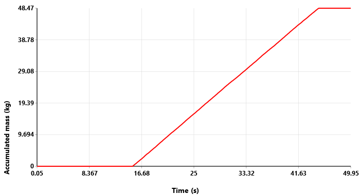
The accumulated mass is the most reliable curve to read the flow rate: being the integral of the instantaneous signal, the pulsation noise vanishes and a straight line remains. Its slope gives about 1.6 kg/s, and it is those ~48 kg discharged that set the total emptying time.
The case simulated in BrixDEM
The case in the video is a discharge of glass beads (mean diameter 13.8 mm, about 14,000 particles) from a 0.5 m tall silo with a hopper whose walls sit at 62.5° and a 57 mm outlet. It is the same configuration as the experimental test of González-Montellano et al. (2011), which lets us confront the simulation with real measurements.
Confronting the experiment
The comparison variable is the total discharge time: since the initial mass is the same, comparing the time is equivalent to comparing the mean flow rate — only much easier to measure. BrixDEM emptied the silo in 29.65 s, against 29.27 s measured in the laboratory (mean of three repetitions).
| Discharge time | Value | Error |
|---|---|---|
| Experiment (González-Montellano et al., 2011) | 29.27 s | reference |
| BrixDEM | 29.65 s | +1.3% |
What else you can extract from a silo model
- Wall pressures: map the peaks at the body–hopper transition that size the structure.
- Dead zones: identify stagnant material (critical for perishable or degrading products).
- Segregation: watch fines and coarse separate during filling and discharge.
- Hopper angle: test how much it shifts between mass flow and funnel flow, without building prototypes.
- Inserts and deflectors: evaluate anti-arching devices before manufacturing.
- Wear: locate where the hopper wall will erode first.
How to reproduce it in BrixDEM
The recipe is short: draw the silo with its hopper in the built-in modeler, calibrate the material (density, stiffness, restitution and friction), fill by gravity until rest, remove the outlet plate and create a measurement region at the discharge. Export the mass flow rate and accumulated mass curves and read the emptying time.
Download BrixDEM and simulate your own silo. See also other simulated equipment and the screw conveyor study, where the same flow-reading logic is applied.
Reference
González-Montellano, C.; Ramírez, Á.; Gallego, E.; Ayuga, F. (2011). Validation and experimental calibration of 3D discrete element models for the simulation of the discharge flow in silos. Chemical Engineering Science, 66(21), 5116–5126. https://doi.org/10.1016/j.ces.2011.07.009
Simulate your own silo
BrixDEM is free to download and runs on Windows. Build the silo and hopper geometry, calibrate the material and read the discharge flow.