
Materials and Contact Interactions
Definition of the mechanical body properties and pairwise contact physics.
10.1 Materials panel
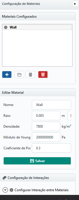
The module Materials shows the list of configured materials and buttons to add, import from database, duplicate and remove. Below the list, an editor allows you to change the properties of the selected material. Further down, Configure Material Interaction defines the pair-by-pair behavior.
10.2 Edit Material
The main fields of a material are:
| FIELD | UNIT | MEANING |
|---|---|---|
| Name | — | Unique material identifier |
| Radius | m | Nominal particle radius (or mean particle size class) |
| Density ρ | kg/m3 | Volumetric density of solid material |
| Young's modulus E | Pa | Longitudinal elastic modulus |
| Poisson's ratio ν | — | Ratio between transverse and longitudinal deformation |
Particle size distribution (PSD)
When PSD is active, the material defines distribution, minimum radius, statistical parameters and a hard maximum radius (PSD Max). The generator uses truncated distribution: no radius produced can exceed PSD Max. The limit should represent the largest physically permitted particle, not just mean + standard deviation.
10.3 Material database
The import button opens a database with common properties as starting values (e.g. sand, ore, steel, glass, polymers). These values are a starting point and shall be calibrated against tests whenever possible - the elastic modulus, in particular, is usually reduced in production to accelerate simulation (see Chapter 20).
10.4 Pairwise interactions
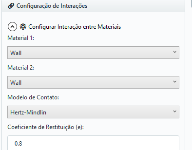
The tab Interactions defines, for each combination of materials, the physical behavior of contact:
| FIELD | MEANING |
|---|---|
| Material 1 / Material 2 | The pair of materials in contact (e.g. ore × wall steel) |
| Contact model | Hertz–Mindlin or Linear Spring–Dashpot |
| Restitution coefficient | - controls normal damping |
| Sliding friction | μ — tangential Coulomb limit |
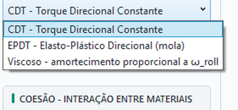
| Rolling friction | μ_r + model (CDT / EPSD / Viscous — Models A/C/B of Ai et al. 2011) — rolling resistance |
| Torsion friction | Marshall (2009) — spin resistance about the normal; uses the pair’s μ, no extra parameter |
| Cohesion | Enable + model (Linear Cohesion / JKR) — attractive force of the pair |
Enabling Rolling friction displays a model selector with the models described in Chapter 3.8. Torsional friction uses Marshall’s model as explained below. The rolling model offers CDT (Model A, constant torque), EPSD (Model C, elastic-plastic spring — stiffness automatic per contact, leave k_r = 0; damping ratio ζ between 0 and 1) and Viscous (Model B, torque proportional to the rolling velocity — uses only μ_r); torsion uses the Marshall (2009) model, with no parameters of its own — the torsional limit coefficient is the pair’s sliding friction itself.
10.5 Contact models available
The models displayed in the interface are Linear Spring–Dashpot and Hertz–Mindlin, both detailed in Chapter 3 (Equations 3.16–3.26). The choice of the model changes the normal stiffness (constant vs. dependent on δn), the energy dissipation in collisions, the characteristic collision time (and consequently the recommended Δt) and the numerical stability in contacts with high overlap.
10.6 Cohesion
Cohesion is switched on by the Enable Cohesion checkbox, following the same pattern as rolling and torsion resistance: unchecked, the pair has no cohesive force and model fields are hidden; checked, you pick the model and enter its parameter. The dry adhesion models, detailed in Chapter 3.9, are: LinearCohesion - additive force F = k·A, compatible with LSD and Hertz, in P–P and P–W - and JKR complete, with adhesion and pull-off, valid only with Hertz–Mindlin. Full JKR can be selected on both P–P and P–W (not wall–wall, which is not a resolved contact), with full pull-off in both cases. The difference is the effective radius: for two equal spheres R_eff = R/2, against a flat wall R_eff = R, so the pull-off force at the wall is double for the same γ.
| STATE / MODEL | WHEN TO USE |
|---|---|
| Cohesion disabled | Dry and non-cohesive granular material (clean sand, crushed ore) |
| LinearCohesion | Moderate adhesion; inexpensive attractive contribution on LSD or Hertz |
| JKR | Fine powders and adhering material: full pull-off in both particle–particle and particle–wall (at the wall, double the force for the same γ) |
| Liquid bridge | Small liquid bridges between surfaces; configure global properties, material content and pair settings in 10.9. Clumps are unsupported. |
Cohesion strongly changes flow, packing and stability. Use carefully and always review Δt when enabling it.
10.7 Coarse-graining
The CGF factor enlarges radii to reduce particle count. At equal total mass and density, each representative stands for approximately CGF³ grains. This is a geometric count estimate; performance gains also depend on timestep, contacts and output. Physical assumptions are in 3.12.
| CGF | Representative radius | Grains represented | Count at equal mass |
|---|---|---|---|
| 1 | R | 1 | N |
| 2 | 2R | 8 | ≈ N/8 |
| 3 | 3R | 27 | ≈ N/27 |
| 5 | 5R | 125 | ≈ N/125 |
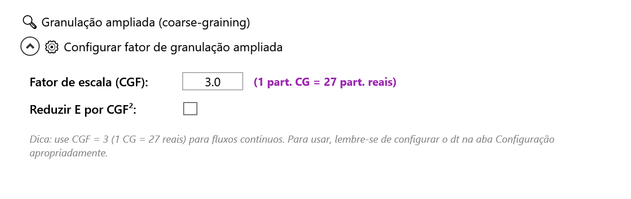
Set CGF first, then check the enlarged PSD and effective timestep in Setup. Mass-based inlets help retain physical flow rate; an unchanged count rate increases introduced mass by approximately CGF³. Adjust the rate and compare the enlarged case with CGF = 1.
E softening and effective pair modulus
The E scaling control is an optional numerical softening. Unchecked (recommended default), it keeps E; checked, it divides E by CGF². The checked option preserves neither E* nor physical contact time. The effective modulus is calculated for each pair:
1/E* = (1−ν₁²)/E₁ + (1−ν₂²)/E₂.
For two identical materials with E = 10 MPa and ν = 0.30, E* = 5.495 MPa. With CGF = 2 and softening applied to both, E becomes 2.5 MPa and E* becomes 1.374 MPa. Check pair overrides separately. E* is a modulus, not the complete incremental Hertz stiffness: stiffness also depends on effective radius and overlap.
| Option | E used | Automatic Rayleigh Δt | Entered fixed Δt |
|---|---|---|---|
| Unchecked | Unchanged | Scales by CGF | Multiplied by CGF in the DLL |
| Checked | E/CGF² | Scales by CGF² | No additional CGF multiplier |
These scalings compare the same original material and radius; free-body limits may reduce the effective step shown. Check Setup after changing CGF or the E option.
Coarse-graining with liquid and breakage
For liquid bridges, enter the original physical properties: the solver scales radii, gap and S₀ by k, surface tension and viscosity by k, and volumes by k³; dry-basis content, density, angle and V/rp³ remain unchanged. For similar geometry and equal surface velocities, force scales by k² and viscous torque by k³. Do not scale GUI inputs again. This does not guarantee preservation of the capillary-to-weight ratio or macroscopic equivalence of every flow. See 3.15 and Appendix H.
For breakage/DWT, keep Young’s modulus consistent with calibration. If E is reduced, apply a consistent reduction to particles and the test wall material, check overrides and recalculate each interaction; changing only one side affects the contacts differently. Recalibrate the energy/fragmentation response and compare CGF = 1 with the enlarged case. Do not automatically transfer a breakage calibration to enlarged particles.
10.8 Composite particles (clumps)
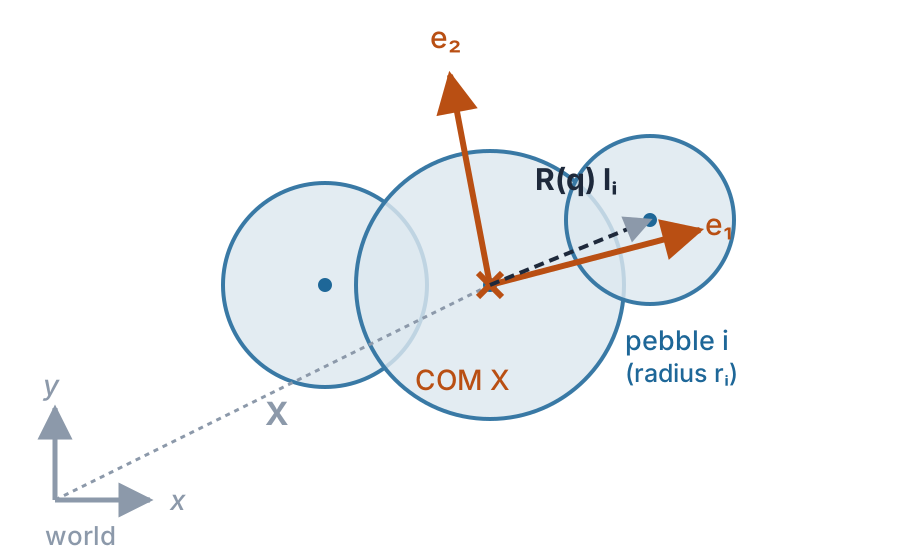
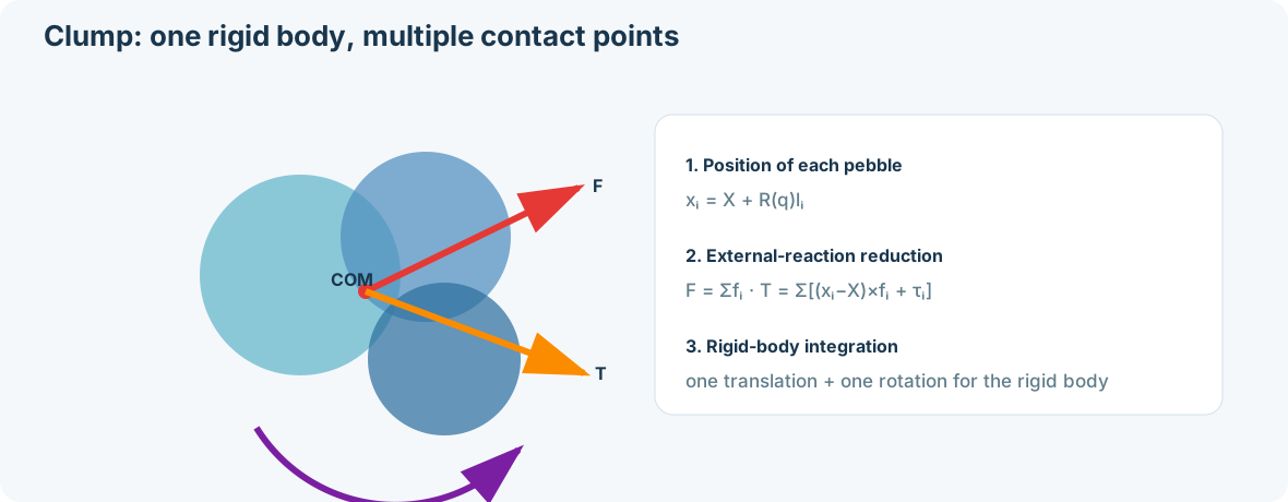
A clump is a rigid particle made of several overlapping spheres ("pebbles") that move and collide as a single body - the right way to represent elongated, flattened or angular grains that a single sphere cannot reproduce. A clump is a material: create it from the 🧩 Define Clump… button on the Materials panel, which opens the clump editor.
Three ways to build a clump
- Presets - ready-made shapes (Capsule, Cylinder, Filled block, Rod, Dimer, Trimer, Tetrahedron, Cube, Disc), parameterized by sphere radius, sphere count, relative overlap (0-0.49) and radius ratio;
- From STL - import a closed mesh and the editor fills the volume with an adaptive sphere packing, controlled by maximum/minimum radius, target overlap and maximum sphere count (mesh unit configurable in mm or m);
- Manual / CSV - edit a sphere table (X, Y, Z, radius) directly, in the clump's local frame, or import a CSV (comma, semicolon or tab separator, auto-detected).
Mass, center of mass and the inertia tensor are computed automatically from the union of spheres (default) or, optionally, from the exact volume/COM/inertia of the original STL solid - density comes from the material. The editor shows in real time: sphere count, mass, equivalent radius, smallest sphere, bounding radius, volume, and (for STL-generated clumps) the coverage fraction of the original mesh.
| LIMIT / RULE | DETAIL |
|---|---|
| At least 1 sphere with radius > 0 | Required to save the clump |
| Maximum of 4096 spheres per template | Limit of the snapshot format (DEM2); the STL generator already caps at 512 regardless of what was requested |
| Maximum of 1024 spheres per template on the GPU backend | Checked when the simulation is assembled: "Clump '{name}' has {N} pebbles; the GPU backend accepts at most 1,024 per template. Reduce the resolution or use CPU" |
| A wall material cannot be a clump | Clumps are exclusive to mobile particles |
| A clump cannot join a multi-material inlet mix | An inlet with a multi-material composition only accepts spherical materials - use a separate, single-material inlet for each clump (Chapter 11) |
| No automatic overlap/connectivity check in Manual/CSV mode | Loose or disconnected spheres are not blocked - the Presets and STL modes guarantee connectivity by construction; in manual mode, it is the user's responsibility |
Features that already work with clumps: particle size distribution (PSD) scaling the whole clump, rolling and torsion friction, and STL surface wear caused by clump impacts. Cohesion (JKR/LinearCohesion) follows the same general pair rule from 10.6 - there is no clump-specific restriction beyond it.
10.9 Liquid bridges
Liquid bridges represent attraction between surfaces joined by small isolated bridges. Theory, the Mikami capillary correlation and Nase viscous resistance are in 3.15. Prepare the case in the following order: liquid properties are global, initial inventory belongs to the material, and the interaction belongs to the pair.
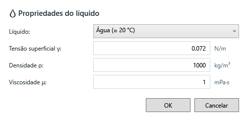
- In the material, open Liquid properties and choose Water, Oil or Custom. Check all three values for the test temperature and composition; the Oil example does not identify a specific product.
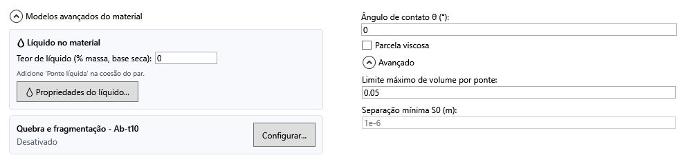
- Enter surface-available Liquid content as a percentage of dry solid mass. Exclude liquid absorbed inside grains.
- In pair interactions, enable cohesion and select Liquid bridge. Content alone does not activate the force. Configure the required particle–particle and particle–wall pairs.
- Set contact angle and optionally enable Viscous contribution. Open Advanced for the bridge limit and S₀.
- Check compatibility in 28.7, timestep in 12.6 and the cases in Appendix H before interpreting the full process.
| Location / field | Unit | Meaning and effect |
|---|---|---|
| Liquid properties · Surface tension γ | N/m | Scales capillary force. Water has a reference value near 0.072 N/m; check temperature. This is not JKR surface energy γ. |
| Liquid properties · Density ρℓ | kg/m³ | Converts liquid mass into available volume. It does not enter the force correlation directly; its effect is through volume. |
| Liquid properties · Viscosity μ | mPa·s in the GUI | Acts only when the pair has its viscous contribution enabled. 1 mPa·s = 0.001 Pa·s; water is approximately 1 mPa·s. |
| Material · Liquid content | % of dry mass | Initial surface inventory. Zero means no initial film, but a prescribed bridge may still provide attraction. |
| Pair · Contact angle θ | degrees | Pair wettability; affects force and rupture. 0° means complete wetting. It is not a friction angle. |
| Pair · Viscous contribution | on/off | Resists normal and tangential relative motion while a bridge exists. Switching it off retains capillary attraction. |
| Advanced · Maximum bridge volume limit | dimensionless: V/rp³ | Default 0.05. With positive content, caps film withdrawal per bridge; with both contents zero, defines prescribed volume. It is neither 5% moisture nor a volume in m³. |
| Advanced · Minimum separation S₀ | m | Regularizes viscous resistance near contact by using a separation of at least S₀. Default 1e−6 m = 1 μm. A smaller S₀ increases near-contact normal resistance; it does not change capillary force or rupture, and does not enable viscosity by itself. |
Dry-basis content and film volume
If w is the entered percentage, initial film volume is Vfilm = (w/100) · mdry solid / ρℓ. Thus 1% means 10 g per kg of dry solid; for liquid density ρℓ = 1000 kg/m³, this is 10 mL per kg. The percentage does not use total mixture mass and does not measure pore saturation. Accepting high content in the interface does not establish validity for coalesced bridges or filled pores.
Prescribed volume and migration
For two spheres, rp = 2 R₁R₂/(R₁+R₂); against a wall, rp is the particle radius. The field defines Vlimit = value · rp³. Two spheres of radius 1 mm with value 0.05 have Vlimit = 5×10⁻¹¹ m³ = 50 nL per bridge at CGF = 1. When both materials have zero content, this is the prescribed volume of each bridge, not an initial moisture balance.
When either material has positive content, bridges draw from available particle films. Competing contacts may receive less than Vlimit; a wall supplies no liquid. At rupture, liquid from migration-mode bridges returns to films. The bridge limit does not cap total inventory or check bridge coalescence. Do not calibrate content solely to obtain a target force: also examine film, bridge and total inventory in Chapter 16.
10.10 Breakage and fragmentation
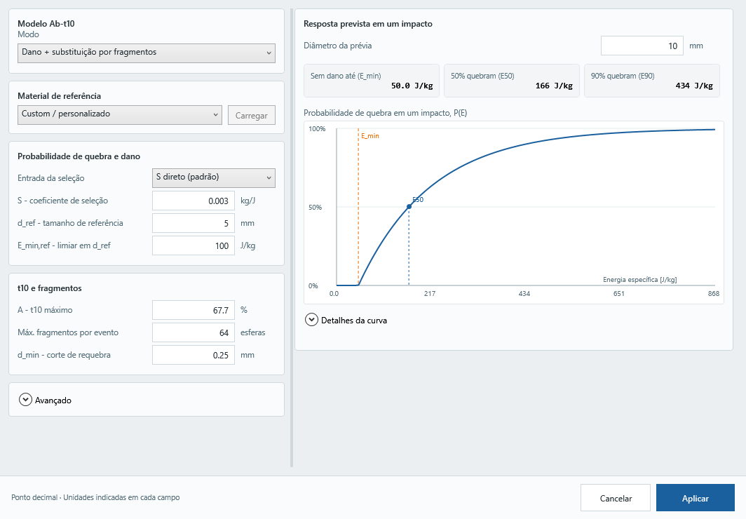
Breakage is configured in the particle material before running the case. Open Breakage and fragmentation, select the Ab-T10/PRM operating mode, enter calibrated parameters, check the preview and timestep and click Apply. Ab-t10 describes selection/damage and t10; PRM replaces the body with fragments. Theory and equations are in 3.16; reproducible verification cases are in Appendix H.
| Field | Unit | Meaning and choice |
|---|---|---|
| Mode | — | Disabled does not calculate breakage; Damage and detection tracks events without replacing the body; Damage + replacement uses PRM and creates spherical fragments. |
| Reference material / Load | — | Selecting an example does not calibrate the case. Load copies the supplied reference parameters; check which fields remain unchanged. |
| Selection input: direct S or JK b + x_ref | kg/J; t/kWh and mm | These represent the same selection law. Use b only with its test size x_ref and protocol; the GUI converts it into S. |
| S — selection coefficient | kg/J | Energy sensitivity at d_ref. Increasing S raises breakage probability under otherwise identical conditions. |
| d_ref | mm | Reference size for S and E_min,ref; it does not change particle geometry. |
| E_min,ref | J/kg | Positive damage threshold at d_ref. At another size d, the threshold scales by d_ref/d. |
| A — maximum t10 | % | Upper limit of mass passing d/10; it is not breakage probability. |
| Maximum fragments per event | 2–64 spheres | Replacement resolution, including the fines representative; more spheres increase cost and change PSD discretization. |
| d_min — rebreakage cutoff | mm | Bodies below the cutoff remain dynamic but cannot break again. Fragments smaller than d_min may be born; this field does not guarantee a minimum timestep radius. |
The breakage dialog explains inputs through tooltips. Material references are optional example presets, not universal calibrations. Custom preserves current values; opening the dialog never loads an example automatically. Calibrate parameters for the material, size, shape and test energy definition.
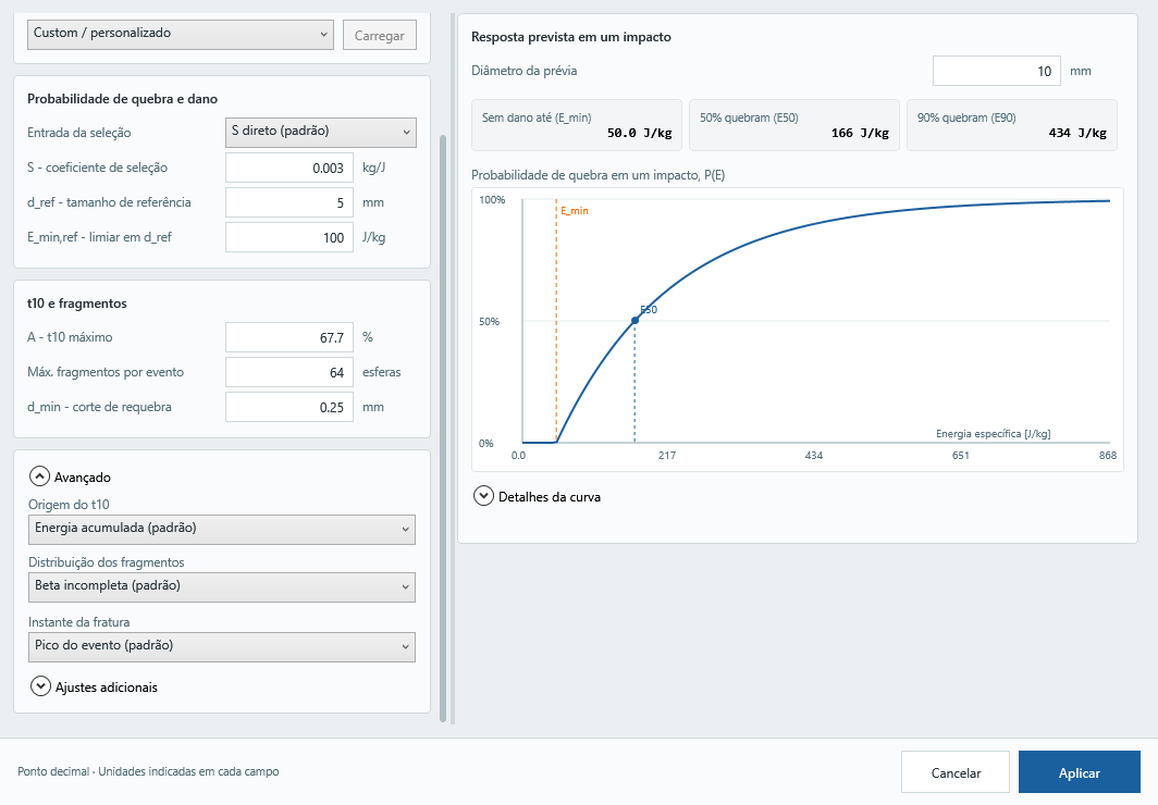
Advanced retains incomplete beta and accumulated-energy t10 as defaults. Event peak and strength crossing are separate choices. Peak also allows early quasi-static fracture with low kinetic energy; crossing need not wait for the peak even in impacts. These choices remain within the Ab-t10 family.
Reference materials: preset sources
The GUI list shows only the material name. This table links each example to its source; selecting a name does not change parameters, and Load copies the available values. Custom retains the current values.
| GUI material | Reference | Adaptation and scope |
|---|---|---|
| Copper ore | Jiménez-Herrera et al. (2018). DOI: 10.1016/j.apt.2017.12.006. | Table 5: copper ore example; the preset values are not a universal calibration. |
| Glass beads | Vogel & Peukert (2004). DOI: 10.1016/j.minpro.2004.07.018. | Master curve adapted to absorbed energy with η = 0.74 for the glass/steel test. The reference does not provide t10: A and fragmentation choices are retained. |
| Rice | Kruszelnicka et al. (2022). DOI: 10.1051/matecconf/202235707005. | Table 4: rice example using Gaudin–Schuhmann and polyhedral particles in the source. The current progeny law and rebreakage cutoff are retained. |
| Coal | Starodubov et al. (2023). DOI: 10.30686/1609-9192-2023-S2-150-154. | Table 2: coal cutting/extraction application; not a universal DWT calibration. |
| Feed pellets | Li et al. (online 2025; 2026). DOI: 10.1080/02726351.2025.2586037. | Section 3.3.3: pellet impacts and pneumatic conveying; the source uses HLS contact. Published online in 2025, volume 44 in 2026. |
Presets are starting points. Check the source energy and test before calibrating your material. Progeny law, resolution, seed and mechanical properties are not imported automatically; d_min changes only when supplied by the preset. Presets do not automatically reproduce the paper or calibrate clumps.
Additional settings
- Damage inheritance: an Ab-t10 PRM option. A fraction of parent exposure, including the breaking event, reduces child strength subject to its floor. Default 0 creates children without inherited damage. This affects subsequent events, not the parent's first fracture. Zero inheritance does not disable damage accumulation within each particle.
- Tangential work fraction: multiplies tangential work added to event energy while the contact compresses. Default 0 uses normal work only. It is not the friction coefficient; positive values change the energy input and require calibration.
- Random seed: determines individual strength draws from seed, particle ID and material. Zero is a valid seed, not a switch disabling randomness. Fix it to repeat strength draws or vary it across statistical replicas. It does not change the analytical mean curve or guarantee identical CPU/GPU trajectories.
Reading the single-impact preview
This is an analytical curve for initially undamaged particles of the same selected diameter, not a virtual DWT or experimental validation. Preview diameter does not change simulation geometry. For clumps it initially uses the volume-equivalent diameter when known, but does not resolve orientation or contacts.
- E_min: event-energy cutoff at the preview diameter; events at or below it cause no damage or fracture. It may differ from E_min,ref.
- E50: single-impact specific energy at which 50% of new particles break statistically, not 50% of each particle's mass or a deterministic threshold for every body.
- E90: analogous energy for 90% breakage probability.
Energy in J/kg means event work per particle mass, not automatically nominal drop energy. Orange marks E_min; blue marks E50. Secondary metrics are under Curve details. t10 describes mass passing one tenth of parent size, not breakage probability; for one impact on a new particle, predicted t10 at E50 equals A/2. The preview does not establish stiffness independence or PRM validation.
For the fracture overlap warning above 50% of radius, Do not ask again during this run suppresses subsequent prompts of that warning after choosing Continue. Counters, CSV, diagnostics and the final summary remain active. The choice resets on the next run; Stop remains the default action. This option does not change the pre-run timestep suggestion.