
Discrete Element Method Theory
Equations of motion, contact geometry, force models and numerical stability criteria used by the BrixDEM solver.
In the Discrete Element Method, each particle is tracked individually and its motion is obtained by explicit integration of Newton's equations. Forces arise mainly from contacts: when two spheres overlap numerically, this overlap is interpreted as local elastic deformation and produces normal and tangential forces. The quality of the simulation depends directly on the choice of material parameters, the contact model and the timestep Δt.
The soft-sphere formulation adopted by BrixDEM follows the classical DEM literature, initiated by Cundall & Strack [1] and consolidated in the contact models of Hertz [2] and Mindlin [3, 4]. Each equation below includes the corresponding primary reference from the scientific literature; the complete list is in Appendix F.
3.1 Equations of motion
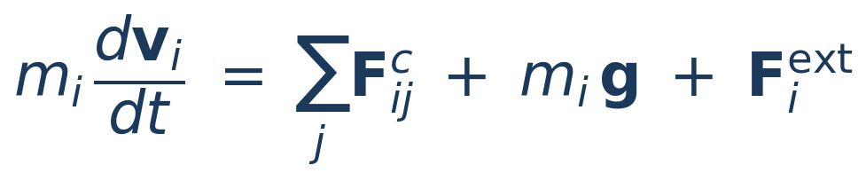
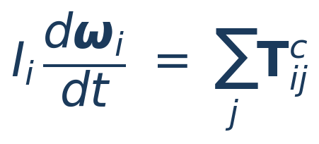
For each particle i of mass mi, radius Ri and moment of inertia Ii, BrixDEM solves linear and angular momentum balances over all active contacts. Integration uses explicit velocity-Verlet integration [18], with normal, relative velocity and tangential history evaluated consistently in particle-particle contact:
 (3.1)
 (3.2)
 (3.3)
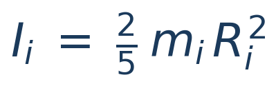
LITERATURE[1] Cundall & Strack (1979) - soft-sphere DEM formulation; [18] Verlet (1967) - explicit integration. Solid sphere moment of inertia I = 2/5 mR2.
Contact forces and torques come from the selected model (Hertz–Mindlin or Linear Spring–Dashpot), summed over all active particle contacts.
3.2 Contact geometry
For two spherical particles i and j, there is contact when the distance between centers is less than the sum of their radii. The vector direction between centers defines the contact normal, which separates the problem into a normal component (compression/restitution) and a tangential (friction/slip).
 (3.4)
 (3.5)
 (3.6)
 (3.7)
LITERATURE[1] Cundall & Strack (1979); [19] Schäfer, Dippel & Wolf (1996) - force schemes and contact kinematics in granular media.
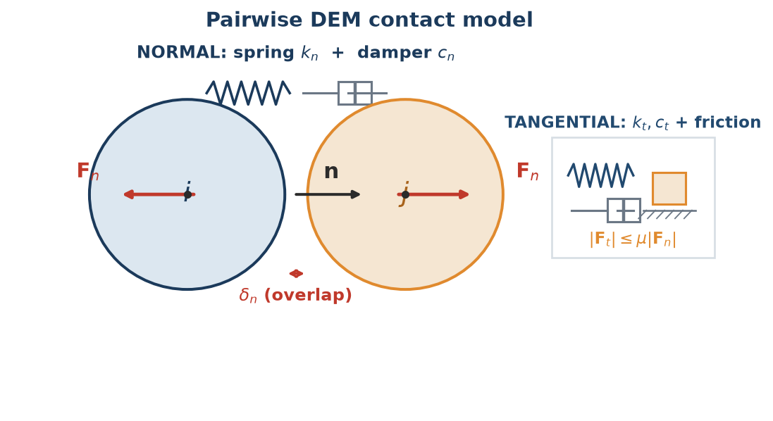
Relative speed includes translation and rotation, correctly capturing shear on the contact surface. The small overlap δn does not represent physical interpenetration - it is the idealized local elastic deformation.
Physical interpretation of contact elements
| ELEMENTS | PHYSICAL MEANING | ASSOCIATED PARAMETER |
|---|---|---|
| Overlap δₙ | Virtual elastic deformation; generates normal repulsion force | Normal stiffness kn |
| Normal relative velocity vn | Approach or separation of particles | Restitution eₙ, damping cₙ |
| Tangential velocity vt | Relative sliding at the contact surface | Friction μ, stiffness kt, damping ct |
| Angular velocity ω | Particle rotation during contact | Rolling μ_r, torsion μ_t |
| Normal force Fn | Compression/repulsion force between bodies | kn, cn, E, ν, δn |
| Tangential force F t | Resists sliding up to the Coulomb limit | μ, k t, c t |
3.3 Restitution coefficient
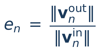
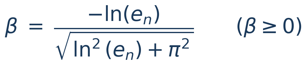
The normal restitution coefficient eₙ measures how much of the normal speed is recovered after impact. The solver uses β ≥ 0 and calculates dissipative coefficients from en; therefore, lower en values produce greater damping:
 (3.8)
 (3.9)
LITERATURE[5] Tsuji, Tanaka & Ishida (1992) - restitution-dependent damping; [6] Di Renzo & Di Maio (2004) - comparison of force models and ratio β(en).
In a simple validation by free fall - a particle falling from height h₁ and rebounding to h₂ in a purely normal collision — the following approximate relation holds:
 (3.10)
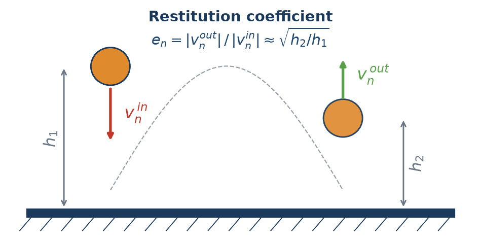
en = 1 represents ideally elastic collision; en = 0, ideally plastic/dissipative. This relationship is useful as a sanity test and is the basis of the rebound calibration assistant (Chapter 18).
3.4 Tangential Friction and Coulomb Limit
The friction configured in the interface acts as contact sliding friction. The tangential model calculates a trial force F_t* that resists the relative slip. As long as this force remains below the Coulomb limit, contact remains in stick; beyond the limit, there is slip.
 (3.11)
 (3.12)
LITERATURE[3] Mindlin (1949); [4] Mindlin & Deresiewicz (1953) - tangential stiffness and contact friction; [1] Cundall & Strack (1979) - Coulomb friction limit in DEM.
Physically, the μ coefficient controls the tendency of the material to slip or adhere. It governs the formation of piles, the angle of repose, shear in chutes and hoppers, and stability in silos and mixers.
3.5 Effective properties of the pair of materials
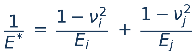
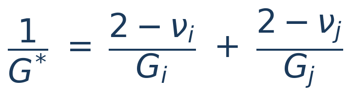
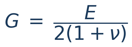
When two bodies interact (particle-particle or particle-wall), the solver uses effective properties calculated from individual properties:
 (3.13)
 (3.14)
 (3.15)
LITERATURE[2] Hertz (1882) - effective modulus E of elastic contact; [3] Mindlin (1949) - effective shear modulus G.
In BrixDEM the contact parameters of the pair - restitution coefficient en, friction μ, rolling friction μ r and torsion μ t - are directly defined for each interaction in the Interactions tab (Chapter 10), and not obtained from mixing rules between materials. The effective geometric and elastic properties above (E, G, R, m) are the natural physical combinations of the pair and are calculated by solver from the properties of each body.
3.6 Hertz–Mindlin model
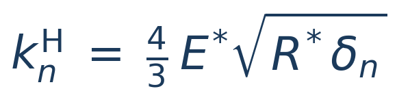
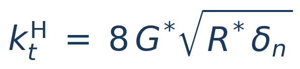
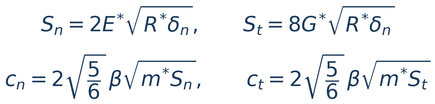
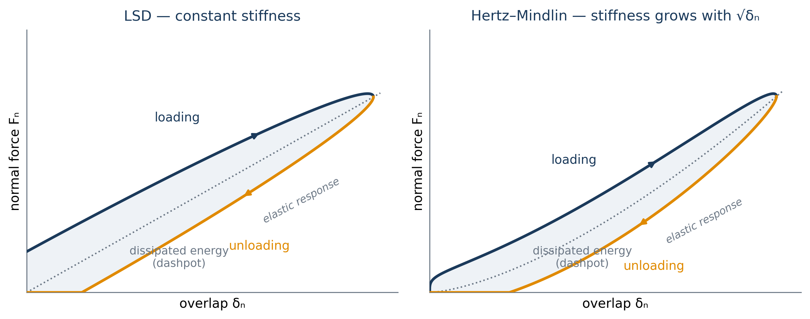
Hertz–Mindlin is a nonlinear model: effective stiffness increases with the square root of overlap δₙ. It is recommended when you want greater physical fidelity in elastic contacts - particularly where the duration of contact and the transmission of force affect the result.
 (3.16)
 (3.17)
 (3.18)
 (3.19)
LITERATURE[2] Hertz (1882) — nonlinear normal stiffness kₙ ∝ √(R*δ); [3] Mindlin (1949) — tangential stiffness; [5] Tsuji et al. (1992) and [6] Di Renzo & Di Maio (2004) — damping based on restitution coefficient eₙ.
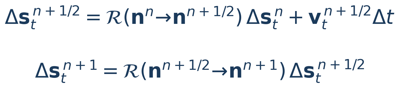
The tangential component uses the history of tangential displacement Δs_t. In particle-particle contact, this history is carried by an objective rotation between the previous and current normals, which preserves its norm when the contact plane rotates and prevents spurious dissipation caused by simple projection:
 (3.20)
 (3.21)
LITERATURE[4] Mindlin & Deresiewicz (1953) - incremental tangential loading with displacement history; [17] Thornton (2015) - objective formulation of contact kinematics.
3.7 Linear Spring–Dashpot model
The Linear Spring–Dashpot (LSD) model uses constant stiffness. It is widely used in calibrations, large industrial simulations and studies where the user wants to directly control stiffness and collision time:
 (3.22)
 (3.23)
LITERATURE[1] Cundall & Strack (1979) - original linear spring–dashpot model; [19] Schäfer, Dippel & Wolf (1996) - linear force schemes.
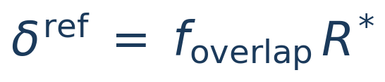
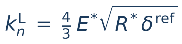
In automatic mode, normal stiffness can be estimated from a Reference overlap user-defined δʳᵉᶠ, calibrating the linear model to reproduce the Hertz–Mindlin contact time. The tangential/normal ratio kt = 2/7 kn is the classic ratio for elastic spheres:
 (3.24)
 (3.25)
 (3.26)
LITERATURE[6] Di Renzo & Di Maio (2004) - equivalent linearisation of Hertz; [16] O'Sullivan & Bray (2004) - choice of stiffness/step; [21] Walton & Braun (1986) - ratio kt = 2/7 kn.
A point in favour of LSD for calibration: in the linear oscillator, the relation between the damping cₙ and the restitution coefficient eₙ (equations 3.9 and 3.26) is exact — the analytic solution of the damped collision — whereas in Hertz–Mindlin the same relation is an approximation. With LSD, the eₙ you configure is exactly the eₙ the normal collision reproduces.
In advanced mode, kn, cn, k t and c t can be entered manually. When defined, manual values prevail over automatic estimates.
3.8 Rolling and torsion resistance
Perfect spheres roll with very little resistance - which produces unrealistic angles of repose and piles that “flow”. To reproduce real angular grains, DEM adds two resistant torques: a rolling resistance (rolling), which opposes relative rolling in the contact plane, and the torsion resistance (torsion), which opposes the spin around normal. BrixDEM implements the three rolling models of the Ai et al. (2011) taxonomy — Model A (CDT), Model B (viscous) and Model C (EPSD) — and one physical torsion model, Marshall (2009), all selectable per pair of materials in the Interactions tab (see Chapter 10).
Common kinematics
Both torques derive from the relative angular velocity of contact, decomposed into a component of rolling (in the contact plane) and a component of spin (along the normal):
 (3.27)
 (3.29)
LITERATURE[11] Ai, Chen, Rotter & Ooi (2011) — taxonomy and assessment of rolling resistance models; [12] Iwashita & Oda (1998) — rolling kinematics at the contact.
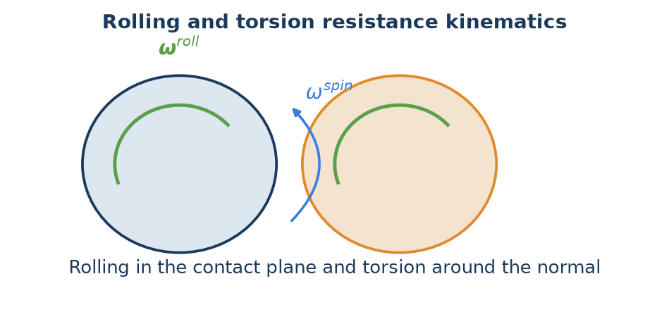
Rolling models
CDT — Constant Directional Torque (Model A of Ai et al.). Applies a resisting torque of constant magnitude, proportional to μ_r, R* and the normal force, always opposing the rolling angular velocity. It is the standard model — robust and cheap:
 (3.28)
LITERATURE[11] Ai et al. (2011) — Model A (Eq. 8a); [20] Zhou et al. (1999) — rolling friction in sandpile formation.
The characteristic limitation of CDT shows up at rest: since the torque has fixed magnitude and only flips sign with the rolling direction, a particle that should stop keeps oscillating around its final position at a frequency set by the time step — torque and friction force flicker between ±M. In dynamic flow this is irrelevant; in quasi-static beds it can contaminate force averages and prevent complete rest (exactly the defect Model C fixes).
EPSD — Elastic-Plastic Spring-Dashpot (Model C of Ai et al., Eqs. 10–20). Accumulates the relative rolling angle θ_r in a torsional spring and applies a torque proportional to that history. While the torque stays below the plastic limit it is reversible (rolling adherence); on reaching the limit μ_r R* ‖Fₙ‖ it saturates by return-mapping (plastic yielding), exactly like tangential friction:
 (3.28a)
 (3.28b)
The rolling stiffness is computed per contact from the normal force — it is not a global number to calibrate. BrixDEM uses the theoretical contact stiffness of Ai et al. (Eq. 7c, after Bardet & Huang) with J_n = ½, which is equivalent to saying that the torque fully mobilises after rolling through a mobilisation angle θ_m = μ_r:
 (3.28d)
Below full mobilisation a critical dashpot with damping ratio ζ (0–1) also acts, dissipating the spring oscillation and allowing complete rest; at full mobilisation the dashpot is switched off (f = 0 in Eq. 17 of Ai et al.). The moment of inertia I_r is that of the rolling vibration mode about the contact point (Ai, Eq. 20) — for a solid sphere each body contributes 7/5 m R²:
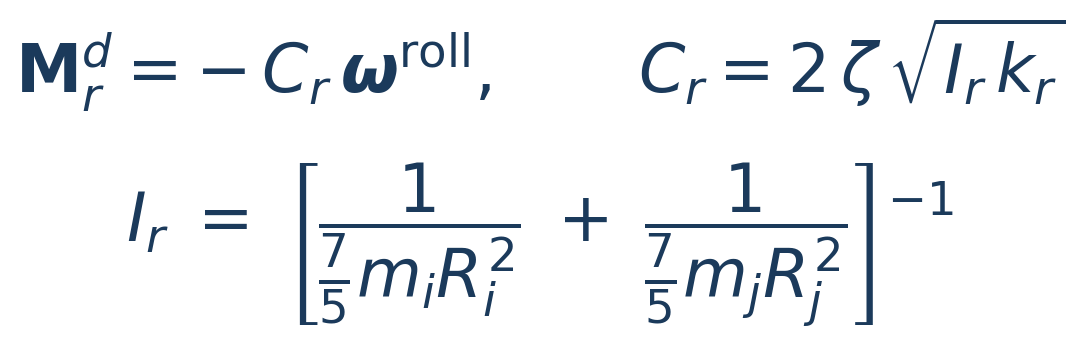 (3.28e)
LITERATURE[11] Ai et al. (2011) — Model C (Eqs. 10–20): elastic-plastic spring with a return-mapping curve, per-contact stiffness and critical dashpot; [12] Iwashita & Oda (1998) — origin of the elastic-plastic rolling model; [13] Wensrich & Katterfeld (2012) — rolling friction as a shape proxy.
Behaviour verified in the solver’s analytic suite: a sphere launched in pure rolling decelerates at a = (5/7)μ_r g, travels d = (7/10)v₀²/(μ_r g) and comes to rest with no residual oscillation; on a ramp inclined less than the resistance angle β = arctan(μ_r) the sphere stays put (Ai, Eq. 1). It is the recommended model for angle of repose, packing and quasi-static regimes. The field k_r > 0 remains available as a manual stiffness override to reproduce older studies; leave k_r = 0 for the automatic stiffness (3.28d).
Viscous (Model B of Ai et al., Eq. 9; proposed by Zhou et al.). Applies a torque proportional to the rolling velocity at the contact surface — the term (R_i ω_i − R_j ω_j), projected onto the contact plane — scaled by the normal force:
 (3.28c)
LITERATURE[11] Ai et al. (2011) — Model B (Eq. 9); [20] Zhou et al. (1999) — original viscous model.
Note the sign combination: for two spheres in mutual rolling (opposite ω) the contributions add and the torque resists rolling; for gear-like spinning (same ω — the surfaces slide) the term vanishes and dissipation is correctly left to tangential friction. For a sphere rolling on a plane the model yields exponential decay, v(t) = v₀·e^(−(5/7)μ_r g t) — with no static threshold. Model B therefore cannot sustain piles nor produce a realistic angle of repose (a conclusion of Ai et al.’s own paper); use it to damp rotations in dynamic regimes, not in quasi-static problems.
Torsion model — Marshall
Torsion resistance uses the formulation of Marshall (2009, Eqs. 29–34): a spring and a dashpot on the relative spin angle θ^spin whose coefficients are not user parameters — they are derived from the tangential contact itself, by integrating the friction traction over the circular contact patch of radius a. The torsional stiffness k_Q and damping η_Q inherit the tangential stiffness k_t and damping c_t of the force model, scaled by a²/2, and the torque saturates at a torsional Coulomb limit with lever arm (2/3)a:
 (3.30)
 (3.31)
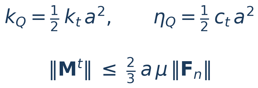 (3.31b)
LITERATURE[14] Marshall (2009) — Eqs. 29–34: k_Q = k_t a²/2, η_Q = c_t a²/2 and M_crit = (2/3)·a·μ‖Fₙ‖ by integrating the friction traction over the patch; [3] Mindlin (1949) — tangential stiffness k_t = 8G*a from which k_Q derives.
The coefficient μ in the limit is the pair’s sliding friction itself: in the paper, F_crit = μ‖Fₙ‖ is the Coulomb critical force of sliding (Eq. 25) and the critical torque results from integrating that traction over the patch (Eq. 33). That is why the interface does not ask for a “torsion μ” — when torsion is enabled, the solver automatically uses the interaction’s μ. Above the limit the contact enters torsional sliding (M = −M_crit along the spin direction, with the same return-mapping as tangential friction); when sliding ceases, the spring k_Q captures the spin and the dashpot η_Q dissipates the residual oscillation. Analytic check: a sphere spinning on a plane decelerates at α = M_crit/I = (5/3)·a·μ·g/R² while sliding, then comes to rest.
Which model to choose
| MODEL | TYPE | PARAMETERS | WHEN TO USE |
|---|---|---|---|
| Rolling · CDT (Model A) | Friction (Coulomb) | μ_r | Default for dynamic flow: piles, drums; oscillates at rest |
| Rolling · EPSD (Model C) | Elastic-plastic spring + dashpot | μ_r, ζ (k_r automatic) | Angle of repose, static packing, quasi-static; rests cleanly |
| Rolling · Viscous (Model B) | Torque ∝ rolling velocity | μ_r | Damp rotations in dynamic regimes; cannot sustain piles |
| Torsion · Marshall | Spring + dashpot derived from the contact | — (uses the pair’s μ) | Dense packing, interlocked grains, torsional shear |
3.9 Cohesion and adhesion
Cohesion adds an attractive normal contribution to the contact, representing van der Waals forces, liquid bridges or surface adhesion. It increases the stability of agglomerates, profoundly changes the flow and, for very sticky materials, requires a smaller Δt. In the additive formulation, the cohesive force is added to the normal contact force:
 (3.32)
LITERATURE[31] Coetzee & Scheffler (2023) — review of DEM cohesion models and their calibration for cohesive materials; [7] Johnson, Kendall & Roberts (1971) — adhesion of elastic solids.
BrixDEM implements two models, chosen by the compatibility with the normal force model:
| MODEL | COMPATIBLE WITH | NATURE | HYSTERESIS |
|---|---|---|---|
| LinearCohesion (linear additive) | LSD and Hertz–Mindlin | Additive force F = k·A, in overlap | No |
| JKR (complete) | Hertz–Mindlin; P–P and P–W (not W–W) | Replaces Hertz normal; full adhesion + pull-off, in P–P and in P–W | Yes |
LinearCohesion — linear additive cohesion
Adds an attractive force proportional to the contact area A — the intersection circle of the two spheres — acting only while there is overlap (δn > 0). It is a simple additive model: cheap, robust and valid for both the linear (LSD) model and Hertz–Mindlin. The parameter k is the cohesion energy density [J/m³] — the larger the compressed area, the stronger the attraction, so cohesion grows smoothly with overlap and vanishes on separation.
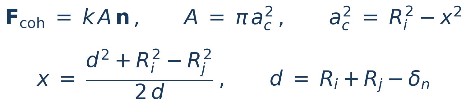 (3.39)
For particle-wall contact, the area uses the sphere–plane formula and the attraction points to the wall:
 (3.40)
LITERATURE[31] Coetzee & Scheffler (2023) — taxonomy of DEM cohesive models (the simplified SJKR F = k·A among them) and calibration from bulk response; [7] Johnson, Kendall & Roberts (1971) — adhesive basis.
JKR — Johnson–Kendall–Roberts (complete)
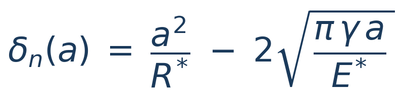
The JKR model replaces the Hertz normal force with an adhesive law parameterized by the contact radius a. Here, a is the radius of the contact circle — the flattened, approximately circular region that forms where the two spheres press against each other. In pure Hertz contact a = √(R*·δn); in JKR the adhesion deforms the edges of that circle (an adhesive “neck” forms) and a is larger than the Hertz value for the same overlap δn. The material parameter is γ, the surface energy [J/m²]: the energy gained per unit area when the two surfaces adhere. The theory follows from the balance between the Hertz elastic energy and the surface term (−γ·πa²), and this competition produces the JKR signatures: a finite contact radius at zero load (a > 0 at δn = 0), sustained tension across an open gap (δn < 0) and a pull-off force on separation. In BrixDEM it can be used on both particle–particle and particle–wall contacts (not wall–wall, which is not a resolved contact) — and both show the full hysteretic behavior: the bond forms at first touch, sustains tension across an already open gap and breaks at pull-off. The only difference between them is the effective radius: for two equal spheres R_eff = R/2, against a flat wall R_eff = R — so the pull-off force at the wall is double that of the particle–particle pair with the same γ (Chapter 28.4; verified in Appendix H, Case 8b). It is recommended for fine powders and cases where elastic adhesion dominates the dynamics. The law is given in parametric form — overlap and force written as functions of a:
 (3.41)
 (3.42)
LITERATURE[7] Johnson, Kendall & Roberts (1971) - original JKR theory (surface energy and adhesive contact).
The adhesive bond only breaks when the traction reaches the pull-off, at a negative distance δ pull (open gap). The inversion a(δₙ) uses the closed-form analytical solution of Parteli & Pöschel (2014):
 (3.43)
LITERATURE[9] Parteli et al. (2014) - closed contact radius a(δ) solution for fine powders; [7] JKR (1971) - pull-off force 3πγR*.
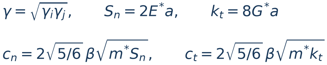
Between different materials, surface energy is combined by geometric mean. Damping comes from the coefficient of restitution eₙ through the Tsuji formulation (β from Eq. 3.9), with normal stiffness evaluated at the actual JKR contact radius, Sₙ = 2E*a. Mindlin tangential stiffness uses the same radius; tangential damping uses the Tsuji form with kₜ:
 (3.44)
LITERATURE[5] Tsuji, Tanaka & Ishida (1992) — restitution-dependent damping; [3] Mindlin (1949) — tangential stiffness using the contact radius.
3.10 Timestep - Rayleigh criterion
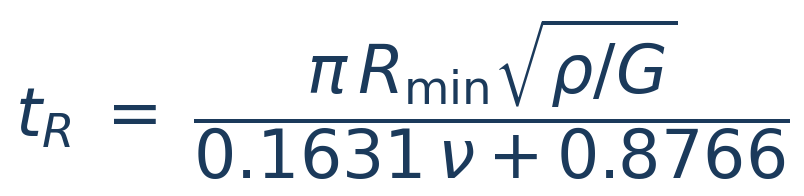
The timestep Δt is one of the most sensitive parameters in DEM. A Δt too large generates excessive overlap, artificial energy, exploding particles and numerical instability. In BrixDEM the automatic calculation of Δt is based exclusively on Rayleigh time - the time for an elastic surface wave to travel through the particle. Solver calculates t R for each particle material and uses the smallest material value, not just the smallest Young's modulus:
 (3.33)
 (3.34)
 (3.35)
LITERATURE[15] Thornton & Randall (1988) — critical time step from the Rayleigh surface wave, with C_R ≈ 0.1631ν + 0.8766.
Automatic timestep
The mode Rayleigh (automatic) applies the α R factor to the shortest Rayleigh time between active materials:
 (3.36)
LITERATURE[15] Thornton & Randall (1988) — Rayleigh criterion; [16] O'Sullivan & Bray (2004) — time-step verification by convergence (their criterion is the mass–spring one, not Rayleigh's). The current automatic mode of BrixDEM uses Rayleigh only.
| SCENARIO | α R INITIAL | RECOMMENDATION |
|---|---|---|
| Simple, monodisperse case | 0,20 | Confirm by Δt convergence |
| Polydisperse, small particles | 0,10–0,15 | Use the smallest radius effectively present |
| Very rigid material | 0,10 | Monitor overlap and kinetic energy |
| Active cohesion (JKR/LinearCohesion) | ≤ 0,10 | Reduce additionally and validate pull-off |
3.11 Contact with walls, STL and primitives
Walls, STL meshes and geometric primitives use the same contact logic as particles: local normal, overlap, relative speed, normal force, tangential force and torques. The difference is that the wall is treated as a fixed or prescribed body, while the particle responds dynamically.
 (3.37)
 (3.38)
LITERATURE[1] Cundall & Strack (1979); [19] Schäfer et al. (1996) - Particle–boundary contact using the same force law; wall treated as a body of infinite mass/radius.
3.12 Coarse-graining: scaling laws
Coarse-graining uses one larger particle to represent a group of grains. Multiplying radius by k at constant density makes representative-particle mass grow as k³. At the same total mass, ideal particle count decreases by k³:
 (3.45)
 (3.46)
These are geometric relations; computing-time reduction also depends on contacts, timestep, output and spatial distribution. In the reference scale with unchanged E, density ρ [kg/m³] and modulus E [Pa] remain constant, as do dimensionless coefficients ν, e and μ:
 (3.47)
For JKR, scaling surface energy γs by k makes pull-off grow as k² because effective radius also grows by k:
 (3.48)
This does not preserve the individual adhesion-to-weight ratio: weight grows as k³ at fixed gravity. Preserving interaction stress, individual Bond number and a trajectory in fixed-size equipment are different similarity objectives. One scaling rule cannot impose all of them without checking its assumptions.
The PSD, including its bounds, is geometrically enlarged:
 (3.49)
At constant ρ and ν, Rayleigh time is proportional to radius and inversely proportional to the square root of E:
 (3.50)
Thus unchanged E gives critical time ×k; E divided by k² gives critical time ×k². This is a contact-stability relation, not proof of process-time equivalence. Optional E reduction softens contacts and requires deformation/calibration checks; its states and the distinction between entered and effective dt are described in 10.7.
LITERATURE[26] — Particle-system similarity laws under scaling assumptions. The reference does not universally justify optional E reduction or equivalence in fixed equipment and gravity.
3.13 Surface wear: physical models
BrixDEM estimates wear of surfaces (chutes, liners, paddles, screens) from the forces and slip of the particle-wall contacts, accumulating the depth removed [m] per mesh triangle. Two physical mechanisms can be combined.
Abrasive wear (Archard)
Models removal proportional to the friction work of sliding contact. Each step accumulates a depth proportional to normal force and sliding displacement, normalized by triangle area (A△). K/H is the specific wear coefficient [1/Pa]:
 (3.51)
LITERATURE[22] Archard (1953) - volume removed proportional to load × sliding distance / hardness.
Impact erosion (Oka)
Models the removal caused by particles that collide with the surface, evaluated at the moment of impact. It depends on impact angle α (function g(α)) and speed v:
 (3.52)
 (3.53)
g(α) describes angular dependence; E90 is the reference erosion at 90°, function of Vickers H v hardness, velocity v and diameter D, with calibrable exponents. The depth is normalized by the area of the triangle and scaled by particle mass.
LITERATURE[23] Oka, Okamura & Yoshida (2005) - predictive equation of impact erosion (angle, speed, hardness); [25] Maw, Barber & Fawcett (1976) - oblique impact of elastic spheres.
3.14 Composite particles (clumps): fundamentals
A clump is a rigid body made of N spheres ("pebbles") of radii rᵢ, with controlled overlap between them, that translate and rotate as a single body - the spheres have no independent degrees of freedom of their own; only the clump as a whole has its own position, orientation, linear velocity and angular velocity. This is how BrixDEM represents non-spherical grains without giving up sphere-sphere contact detection, which is cheap and robust.
Mass properties
The clump's mass, center of mass and inertia tensor come from the geometric union of the N spheres - not from the naive sum, which would count the overlap region twice: the volume is integrated numerically (voxelization) over the composite shape and multiplied by the material density. The center of mass is the volume-weighted average, and the inertia tensor uses the parallel-axis theorem to shift each sphere's own inertia to the clump's center of mass:
 (3.54)
where dᵢ is the distance from sphere i's center to the clump's center of mass (the overlap between spheres is already accounted for by the voxelization). Alternatively, BrixDEM can compute mass/COM/inertia from the exact STL solid that generated the clump, when available (10.8) - more accurate for shapes with substantial overlap, at the cost of requiring a closed mesh.
Contact and integration
Each pebble takes part in contact detection normally, as if it were an ordinary spherical particle - against other particles, against other clumps, and against walls/STL. The difference is in the integration: instead of each pebble receiving its own linear and angular acceleration, the forces and torques from every contact of every pebble in the clump are summed and applied to the single rigid body (using each pebble's position relative to the center of mass as the torque's lever arm). The result is integrated once per clump, not once per pebble - the clump advances in time as the large, rigid particle it represents, and the spheres simply follow that kinematics, rigid with respect to each other.
3.15 Liquid bridges
A small amount of liquid outside a grain can form a meniscus between contacting surfaces. Pressure difference and surface tension create attraction; relative motion can also dissipate energy through viscosity. BrixDEM uses the Mikami correlation for attraction and rupture distance, with optional normal and tangential resistance from the Nase viscous approximation. A bridge forms at contact, remains during separation and ruptures beyond its critical distance. Proximity alone, without prior bridge formation, does not mean that a bridge is active.
Geometry, units and conventions
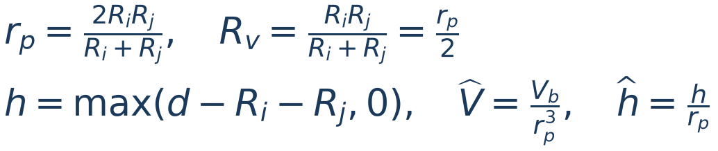
Consider spheres with radii Rᵢ and Rⱼ, center distance d and bridge volume Vb [m³]. The capillary radius rp differs from the lubrication radius Rv:
 (3.55)
h [m] is the nonnegative gap: the capillary correlation uses h = 0 during overlap. For sphere–wall contact, use rp = Rv = R, the sphere radius. Surface tension γl is in N/m; θ is converted from degrees in the GUI to radians in the equations. Do not confuse γl with the surface-energy parameter of the JKR model.
Capillary force and rupture
The attractive-force magnitude follows the expression below. Its direction points toward the other surface, with an equal and opposite reaction on the other body.
 (3.56)
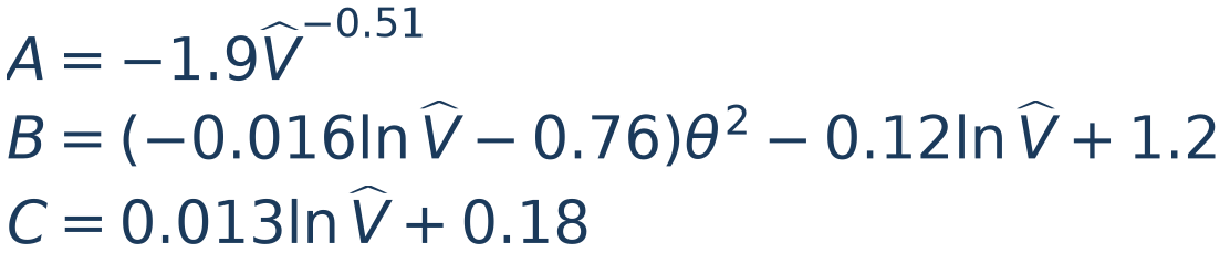
For sphere–sphere contact, the coefficients depend on dimensionless bridge volume:
 (3.57)
For sphere–wall contact, with V̂ = Vb/R³ and ĥ = h/R, use:
 (3.58)
Do not add an external cos θ factor: angular dependence is already included in the published coefficients, including θ². An existing bridge stops acting when h exceeds its critical distance:
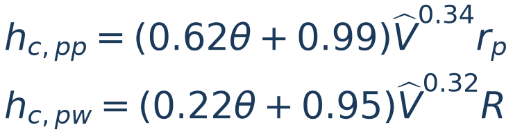 (3.59)
LITERATURE[32] — Mikami, Kamiya & Horio (1998), force and rupture correlations, Eqs. 22–25. Unequal spheres use rₚ; walls use their own correlation.
Viscous contribution and minimum separation
When enabled, viscous resistance uses dynamic viscosity η [Pa·s]; the GUI accepts mPa·s, with 1 mPa·s = 10⁻³ Pa·s. S₀ [m] regularizes nearly touching surfaces:
 (3.60)
cn and ct have units N·s/m. Using relative surface velocity and unit normal n, viscous force opposes motion:
 (3.61)
Tangential velocity includes surface rotation. The tangential contribution also produces torque through the contact lever arm. The nonnegative logarithmic factor prevents a tangential force that supplies energy outside the asymptotic approximation. Decreasing S₀ increases normal resistance near contact; it does not change static capillary force or rupture distance. At zero relative velocity, viscous force is zero.
LITERATURE[33] — Nase et al. (2001), near-contact viscous resistance. Minimum separation and the nonnegative bracket are implementation regularizations.
Liquid content, surface inventory and volume modes
GUI liquid content w is a percentage of dry-solid mass md, rather than void volume or mixture mass. Liquid density ρl [kg/m³] converts initial liquid mass to film volume:
 (3.62)
Thus 1% means 10 g/kg dry solid. A sphere with R = 1 mm and ρs = 2,500 kg/m³ has dry mass 1.04720 × 10⁻⁵ kg; with water density 1,000 kg/m³ and 1% content, its initial inventory is 1.04720 × 10⁻¹⁰ m³. Film is a scalar available reserve, not a resolved three-dimensional coating or liquid absorbed inside the grain.
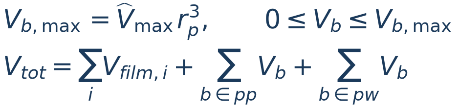
Prescribed volume: when both material contents are zero, the pair specifies volume per bridge through the relative value. Migration: when content is positive, liquid comes from films; the same relative value limits what each bridge can receive, subject to inventory and competing contacts. A wall receives liquid from the particle and has no donating inventory.
 (3.63)
The sum counts each bridge once, including wall bridges. In a closed system with inventory, formation and rupture redistribute liquid between films and bridges; Vtot should remain constant within numerical tolerance. For an open system, include introduced and removed liquid. Prescribed mode does not represent a conserved moisture inventory: bridge count can change without a surface reserve supplying it. A limit V̂max = 0.05 means neither 5% liquid content nor a universal saturation boundary.
Coarse-graining and validity
For local geometric similarity, the adopted parameter scaling preserves dimensionless arguments of the correlation and makes interaction forces grow as k²:
 (3.64)
These relations require the same angle, volume scaled by k³ and identical relative surface velocities. Preserving surface speed in a rotating initial condition requires ω to scale as 1/k; the input does not apply that conversion automatically. Enter physical properties in the GUI: do not manually multiply γl or η before applying CGF. Liquid content, liquid density and V̂max remain unchanged.
LITERATURE[38], [39] — Larijani, Magnanimo & Luding (2025) support parameter scaling for k² interaction forces. Chan & Washino (2018) use a different strategy, evaluating at original scale before an external multiplier; the implementations are not identical.
3.16 Breakage and fragmentation
A breakage description separates three questions: which body reaches fracture, what damage remains after a non-fracturing event, and how mass is distributed among products. Ab-T10 describes selection, damage and t10; the Particle Replacement Method (PRM) replaces the fractured particle with discrete fragments. PRM is a replacement strategy, not an independent mineral-strength law.
Event energy and partition between bodies
An event groups loading of a body by its contacts. Energy input is assigned contact work divided by body mass; it is not automatically nominal drop-weight energy mgh, machine kinetic energy, or the instantaneous “Impact energy” scalar. The implementation accumulates normal and, when selected, tangential work increments:
 (3.65)
Fn+ is compressive normal force, Δδ is the overlap change and ΔWt is tangential work computed during loading. cs is the tangential fraction included in body breakage. Partition χ uses each material’s Hertzian stiffness [Pa]; it is 1/2 for equally stiff bodies. Normal work is signed through the contact cycle and the event retains the loading peak; summing absolute increments would define a different energy.
Fracture decision can use the event peak/end or resistance crossing during loading. Dialog choices and early decision under quasi-static compression are detailed in 10.10. Energy reached at the decision affects t10 and progeny; different protocols therefore do not automatically share calibrated parameters.
LITERATURE[36], [37] — Fracture energy, elastic partition and loading events. Event discretization and replacement timing must be kept consistent when reproducing a calibration.
Ab-T10: size, probability and accumulated damage
Let d [m] be representative diameter; dry clumps use volume-equivalent diameter. S [kg/J], dref [m] and emin,ref [J/kg] define the size-dependent selection coefficient and cutoff:
 (3.66)
For new particles of identical size under one impact with specific energy e [J/kg], breakage probability is P₁. Across successive events, net exposure sums the part above the cutoff:
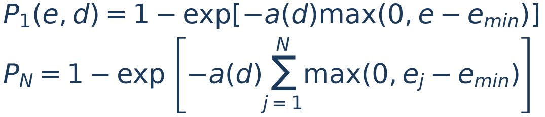 (3.67)
P is a population fraction, not the fraction of mass fragmented within one particle. Each body receives one initial sampled threshold. When an event does not fracture it, damage reduces remaining resistance:
 (3.68)
The body fractures when eevt reaches its remaining threshold. An event below emin does not lower that threshold. A new independent resistance is not sampled at every collision. Optional inheritance applies a fraction of prior parent exposure to children, subject to the model floor; zero inheritance does not disable the body’s own damage accumulation.
LITERATURE[34], [35] — Vogel–Peukert energy/size selection and Shi–Kojovic size–energy relation; the equations show BrixDEM parameterization and accumulation.
Ab-T10: t10, reference energy and curve preview
GUI parameter A is a percentage; M = A/100 is its fractional form. At fracture, net energy can include prior accumulated exposure H or only the breaking event:
 (3.69)
H = T₀ − Told for accumulated energy and H = 0 for event-only energy. A changes the t10 limit without changing P₁. For a new population, the single-impact preview gives:
 (3.70)
e₅₀ is the energy at which 50% of a new population breaks, not deterministic strength of each body. At this point, single-impact predicted t10 is A/2. Prior damage and size changes invalidate this direct interpretation. The alternative JK b and xref representation converts as:
 (3.71)
xref and dref must use the same length unit. The 3,600 factor converts kWh/t to J/kg; entering b as if it were S changes the energy scale. The preview checks parameterization but is not experimental validation.
Progeny and PRM replacement
t10 is mass passing an aperture equal to one tenth of parent size. Distinguish t10, breakage probability and child count. The incomplete-beta family relates t10 to other tn markers:
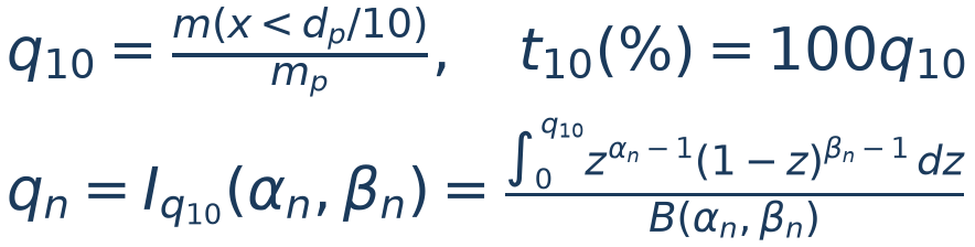 (3.72)
αn and βn are dimensionless, material-dependent parameters. The solver interpolates points logarithmically and enforces anchor Q(0.1) = q₁₀. The Gaudin–Schuhmann alternative uses the same anchor with a power curve:
 (3.73)
A finite set of fragments and, where applicable, fines representatives discretize the continuous distribution. Maximum fragments controls resolution and cost. A rebreakage cutoff does not guarantee that no smaller child can be born; see the Ab-T10/PRM rule in 10.10. Mass accounting includes fines:
 (3.74)
Replacement must conserve mass, with momentum transfer and initial separation verified. Collision-peak energy should not be interpreted as energy entirely recovered in child motion. Agreement of mass/t10 verifies discretization; experimental PSD comparison assesses material representation.
LITERATURE[36], [37] — Incomplete-beta distributions and stochastic particle replacement; conservation rules and evidence are in Appendix H.