
2D Plots and Results
Time series plotting (energy, counting, forces, flow) and quantitative analysis.
16.1 2D Plots tab
The tab 2D Charts plots results of CSV files and selected variables. The panel Results offers quick variables for the main results and an advanced X–Y plotter. Each graph can be configured with title, axes, limits, line color and legend, and exported as CSV or PNG.
16.2. Results and variables panel
Select a variable in Results and click 📈. For rows with μ / min / max, first choose the statistic. At each saved time, μ is the arithmetic mean of the available individual values; min and max are population extremes at that time, not extremes over the entire run. Global quantities such as total mass have no such selector. Compare cases using the same population, units and output interval.
| Group | Plots and basis |
|---|---|
| Energy | KE, PE and TE, global quantities in J (16.3). |
| Particles | N, packing fraction φ, |v|, |ω|, |F|, residence time, radius, total mass, impact energy and compression force. Individual variables support mean/min/max; total mass is global. |
| Contacts | Total contacts, contacting neighbours and relative overlap; global count or population statistics according to the row. |
| Geometries | Force, torque, power and enabled wear; per-geometry results and summaries of copies (16.4 and 16.10). |
| Outlets and monitors | Rates, cumulative values, inventory and regional properties (16.5, 16.8 and 16.9). |
| Mixing | Lacey and concentration CV, with the number/mass/volume basis available for each metric (16.6). |
| Liquid bridges | Film, bridge and total liquid volumes; mean free content per material (16.11). |
| Breakage | Fractures, attrition, event work, fines, size distribution and body diagnostics (16.12). |
| Free bodies | Position, orientation, velocities, force, torque and power of freely moving STL bodies (16.13). |
16.2.1 Reading particle plots
| Variable and unit | Meaning and use |
|---|---|
| N [count] | Population represented in particle output at that time. Feeding, removal and fragment replacement change N; more particles do not necessarily mean more mass. |
| φ [dimensionless] | For particle aggregation: Σ(4πr³/3)/Vdomain. This is a global indicator relative to the configured domain, not local bed porosity. A clump sphere representation can include overlapping volumes; this value is not the exact geometric solid volume. |
| |v| [m/s] and |ω| [rad/s] | Linear and angular speed magnitudes. The mean of magnitudes is not the magnitude of a mean vector; opposite motions do not cancel. Saved maxima can miss motion between output times. |
| |F| [N] | Magnitude of each recorded force vector. Opposite forces can cancel in this resultant; it is not the sum of compressive normal loads. |
| Residence time [s] | In GUI aggregation, t − tfirst observation of ID. This measures observed age in the available history. A file starting after injection cannot recover earlier time; it is not time remaining until discharge. |
| Radius [m] | Sizes represented in the saved population. A number mean is sensitive to newly generated fines; use the dedicated mass-based PSD for product grading. |
| Total mass [kg] | Sum of recorded masses at a time (mean mass × N). Combine it with inlet/outlet mass and model fines for a balance consistent with saved representation. |
| Impact energy [J] | Eimp,i = Σc ½meff,cvn,c² over retained compressive contacts of a body at the sampled step. meff is normal effective mass and vn is relative normal velocity. Values can also occur during unloading. This is instantaneous normal kinetic intensity, not absorbed work, dissipation, accumulated event energy or a historical peak. |
| Compression force [N] | Fcomp,i = Σc Fn,c+, a scalar sum of retained compressive normal forces, excluding cohesive attraction. Two opposite 10 N forces give zero resultant but 20 N compression. Use it to compare loading levels and identify highly loaded bodies. |
Impact energy and compression force belong to Particles and use min/mean/max from particle_diagnostics_summary.csv. Contact-free mobile bodies contribute zero and clumps count once in this diagnostic. A mean can decrease because more bodies have no contact. To locate a peak, compare with the corresponding 3D scalar at the same time.
16.2.2 Contacts and discretization quality
Total contacts counts recorded contacts at a time. Contacting neighbours describes particle coordination; its mean helps distinguish dispersed flow from a dense network, but depends on shape and wall contacts. Relative overlap is penetration normalized by the diagnostic reference radius, in %. Use its maximum to detect excessively deformed contacts: a mean can hide a few critical contacts. Compare the same radius definition and representation across cases.
Time resolution follows the source output files. A maximum across particles at a saved time is not the maximum between saves. Missing or unavailable fields do not mean zero. The advanced plotter can inspect other saved columns but cannot recover data that were never recorded.
16.3 Energy
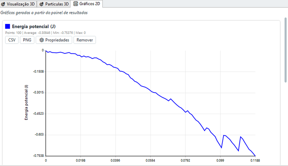
energy.csv contains step,time,KE,PE,TE. KE includes translation and rotation: KE = Σ[½m|v|² + ½ωTIω]. I is scalar for spheres; clumps use rigid-body energy without adding constituent spheres again. PE = −Σm g·x is gravitational potential energy relative to the coordinate origin. TE = KE + PE, in J.
TE is not a complete equipment energy balance: it does not automatically add contact elastic energy, drive work, cumulative dissipation or fracture energy. Inlets and outlets transport energy. A moving wall can physically increase KE; a falling body loses PE and gains KE before contact losses. Assess stability using operating conditions, contacts and timestep together; increasing KE alone does not demonstrate a numerical error.
During settling, KE near zero indicates little motion. Flow and mixing can instead reach a fluctuating plateau. Compare time-window averages in steady operation and assess sensitivity to output interval.
16.4 Geometry results
Enable measurement on a geometry to record its force and torque in body_forces.csv. Quick plots use resultant magnitudes |F| [N] and |T| [N·m]; the advanced plotter can select signed components. A magnitude gives intensity, while a component reveals direction and reversal. Interpret torque about its configured reference point/axis, not solely from STL shape.
Use force for transmitted surface loading and torque/power for drive comparison. Account separately for self-weight or external mechanical losses when they are not included in the recorded result. “Copies (min/mean/max)” compares copies at the same time, not values across time.
Enabled wear adds abrasion, impact and total wear-depth curves, in m. Min/mean/max describe the recorded surface-element distribution; the mean is not automatically total lost volume. Depth [m] is not removed volume [m³]: conversion requires areas and the surface distribution. Calibrate wear coefficients before estimating service life.
16.5 Flow per outlet
Each outlet provides particle rate [part/s], mass rate [kg/s], cumulative particle count and cumulative discharged mass [kg]. Rates describe passage per measurement interval, not a continuously known flux between samples. In steady flow, cumulative mass approaches a straight line whose slope is mass rate.
Use mass rate for throughput and number rate for entity frequency. Breakage can increase part/s through small fragments without increasing kg/s. For a window [t₁,t₂], calculate [Mcum(t₂) − Mcum(t₁)]/(t₂−t₁); separate startup from steady operation. Outlet removal changes domain inventory.
16.6. Mixing index
For two or more particle species, the GUI calculates mixing indices on demand from available snapshots using adaptive spatial binning (cells containing a few dozen particles). Results are written to mixing.csv:
- Lacey Index - uses 0 as the segregated reference and 1 as the random-mixture reference; it is a classical mixing-quality metric;
- Concentration CV - coefficient of variation of the fraction of a species between cells; the smaller, the more homogeneous the mixture.
Use the Lacey time curve to compare drum, V and ribbon mixers. Growth followed by a plateau can indicate a steady mixing condition, subject to the sampling limitations below. Compare geometry and operating time using the same sampling scale.
16.6.1. How to read the Lacey chart
For a species with number fraction p, M = (σ₀² − σ²)/(σ₀² − σᵣ²), where σ₀² = p(1−p), σᵣ² = p(1−p)/n̄ and σ² is the spatial variance of concentrations in valid cells. n̄ is their mean occupancy. The random reference includes finite-count fluctuations; M is therefore not simply a “percentage mixed”. Compare cases with equivalent spatial sampling.
The chart shows one curve per material and, when three or more species are present, two dashed aggregate curves:
| Curve | What it represents |
|---|---|
| Material X vs. rest | Index of material X measured against all the others combined (one-versus-rest). It is not a comparison between two materials. |
| Composite OVR index (dashed) | Average of the per-material indices, weighted by number fraction. Summarises the mixture in a single number. |
| Lowest OVR Lacey (dashed) | The worst material at each instant. A conservative criterion: the mixture is only ready once this curve rises. |
With only two species a single curve appears, labelled with the pair (A × B). This is not an omission: in a binary mixture the concentration of one species determines the other, and both indices are mathematically identical — the second curve would lie exactly on top of the first.
Value range. The Y axis always includes the reference interval [0, 1], but the value is not clamped. A slightly negative index means the material is more concentrated than the segregated reference state (usually an effect of the sampling scale); above 1 means lower variance than a random mixture, which is possible in very regular arrangements. Both are diagnostic information, not calculation errors.
When the curves bunch together. Mixtures that reach steady state quickly live between 0.94 and 1.00 — that is, in the top few percent of the chart. Use ⚙ Properties to set the lower Y-axis limit (0.90, for example) and separate the curves visually.
16.6.2. How to read the concentration CV
CV = σc/μc, with mean and standard deviation of concentration across valid cells on the selected basis. It is dimensionless. CV = 0 indicates equal sampled cell concentrations; larger values indicate more variation. If the species is absent, do not interpret a degenerate division as perfect mixing.
The CV is computed per material — it is the spatial dispersion of that species' concentration, not a comparison between species. Lower is better, and the value has no upper bound. There are three bases:
| Basis | Column | When to use it |
|---|---|---|
| Number | cv_number | The default. When the particle count of each species is what matters. |
| Mass | cv_mass | Polydisperse mixtures or density contrast, and whenever the batch composition is specified by mass. |
| Volume | cv_volume | When occupied volume better represents the composition. |
cv_mass and cv_volume return exactly the same value at every instant, it is because all materials share the same density: mass is then proportional to volume and the two bases coincide. That is the expected result, not a defect.16.6.3. Sampling quality
The metric is measured on a Cartesian grid over the domain and only uses cells with enough particles. Above the chart BrixDEM shows the sampling diagnostics: valid cells, mean occupancy and the count of discarded samples. Read those numbers before drawing any conclusion from the curve — too coarse a grid hides segregation, too fine a grid produces invalid cells and noise.
Breaks in the curve. When an instant could not be measured (insufficient cells, or a degenerate fraction for one material), the line is broken instead of crossing the gap. A blank stretch means no measurement, not a zero value. Isolated measurements between two gaps appear as a single dot.
LITERATURE[24] Lacey (1954) - particle mixing theory and definition of the mixing index (variance between samples normalized by segregated and random states).
16.7 Advanced plotter and graph properties
The advanced plotter allows you to choose the source file (any CSV generated by the solver), the X axis (usually time or step), multiple overlapping Y series and style (line, scatter, markers).
| PROPERTY | RECOMMENDATION |
|---|---|
| Title | Content description (e.g.: "Torque of the drum - case A") |
| Axis labels | Include units in brackets - e.g.: t [s], τ [N·m] |
| Limits | Set manually for case comparison |
| Line colour | Different colors for multiple series |
| Grid / Legend | Enable grid for quantitative reading; show a legend whenever there is more than one series |
Overlay series with compatible units and scales. Use time [s] for physical comparison; step counts increments and is not the same physical time across runs with different timesteps. Distinguish a population statistic at each instant from the time average of a curve. For files with multiple entities or materials, check filters and legend before interpreting a line. Export preserves available samples and cannot recover intervening peaks.
16.8 Region monitors (measurement without removal)
One region monitor measures what passes or remains in a region of the domain without removing the particles - different from an outlet, which discards them. It's the tool to instrument a simulation as if it were virtual sensors. The region may be a plane (counts what crosses it, in one or both directions) or a box (measures content within volume).
| MEASURED QUANTITY | WHAT IT REVEALS |
|---|---|
| Count and mass | How many particles / how much mass cross the plane or are in the box (flow) |
| Time of residence | How long ago the particles were injected (mixture, dead zones) |
| Kinetic energy | Agitation of the material in the region |
| Speed | Average/max speed of material passing or residing |
| Size (radius/diameter) | Local granulometry - flow breakdown by size class |
| Angular velocity ω | Rolling/spinning in the region |
| Force | Load on material in the region |
For monitors, count_inside and mass_inside_kg are instantaneous inventory [particles and kg]; entry/exit rates are fluxes [part/s], while cumulative values count crossings. Repeated crossings need not be unique IDs. Mean/min/max residence [s] concerns monitored episodes, not fragment age. Total/mean KE [J], mean/max speed [m/s], mean/min/max diameter [m], mean/max angular speed [rad/s] and mean/max force [N] describe the population sampled in the region. Check occupancy and availability before comparing means: an empty region does not measure a zero material property.
16.9 Flow per size class
Combining the monitor with reading of size, it is possible to separate the flow rate by particle size range. This is essential to evaluate screening (as each class passes through the deck) and segregation (whether fine and coarse particles separate along the equipment). With a PSD in the inlet (Chapter 11.6), compare the distribution that enters with the one that crosses each monitor.
Size-class curves use the monitor’s configured limits: number rate [part/s], mass rate [kg/s], count [particles] or mass [kg] per class, according to available columns. Per-class curves are differential distributions, unlike the cumulative mass-passing plot under Breakage. For comparison with experimental grading, use the same mass/number basis, sieve limits and passage/inventory population.
16.10 Torque and mechanical power by geometry
For moving bodies (drums, mixers, paddles, belts), the file body_forces.csv records, in addition to force and torque, the angular velocity and mechanical power P mech consumed by the body to move the material:
| COLUMN | MEANING |
|---|---|
| Fx, Fy, Fz, F mag | Resultant force on the body and its magnitude [N] |
| Tx, Ty, Tz, T mag | Resultant torque and its magnitude [N·m] |
| omega | Angular velocity of the body [rad/s] |
| P mech | Mechanical power = T·ω [W] - energy per second to move the material |
body_forces.csv (Fx,Fy,Fz,F mag,Tx,Ty,Tz,T mag,omega,P mech) - generated for each geometry with measurement enabled.16.11 Liquid-bridge post-processing
Liquid bridges appears when a material pair is configured with this model. Select Liquid volume (m³) to overlay films, bridges and total from liquid_bridge.csv. In inventory mode, Vtotal = Vfilms + Vbridges; bridges to walls are included.
| Curve | Interpretation |
|---|---|
| Films [m³] | Liquid available on surfaces. A decrease can mean transfer into bridges without loss of total liquid. |
| Bridges [m³] | Liquid allocated to active bridges. Growth with decreasing film volume indicates redistribution; rupture can return liquid to inventory. |
| Total [m³] | Accounted inventory. Inlets and outlets can change this total in an open domain. |
| Mean free content per material [%] | 100ρlΣVfilm,i/Σmdry,i over that material. This dry-mass-weighted mean excludes bridge liquid and is not total bed liquid content. |
A free content of 1% means 10 g of available liquid per kg of dry solid. Compare materials on the same dry-mass basis. Many small particles do not receive extra weight merely because there are more of them. Without particles of that material or the saved field, the result is unavailable.
Inventory curves have physical accounting meaning in the liquid-stock/migration mode; prescribed volume per bridge alone is not a conservative reservoir. Do not infer evaporation or liquid creation from a single curve. Check films + bridges together with boundary flows. Older files may lack these fields; plots do not validate unsupported model combinations.
16.12 Breakage results
Breakage contains global results and body diagnostics. Rows depend on available files; enabling a model does not reconstruct missing history. Use time series for rates and balances, and distribution plots for event work and particle size.
| Plot / unit | Basis and engineering interpretation |
|---|---|
| Fracture rate [s⁻¹] and cumulative fractures [count] | The rate gives frequency per interval; the cumulative count records fracture/replacement events. One fracture producing several children is one event. |
| Mass processed in fractures [kg] | Sums fractured-body mass, including repeated breakage. The same material can be counted several times; this is not unique converted mass or discharged mass. |
| Cumulative attrited mass by material [kg] | Removal attributed to attrition by the model. Distinguish it from resolved-fragment mass and inventory size distribution. |
| Event-work distribution [count per J range] | X: positive recorded-work ranges; Y: event count, including events without fracture. Describes loading exposure, not instantaneous impact kinetic energy or total equipment input energy. |
| Cumulative model fines [kg] | Fines predicted by the model according to saved representation. Unresolved fines are not necessarily visible particles; distinguish model prediction from explicit population. |
| Size distribution — initial/current inventory [mass passing fraction] | X: size; Y: cumulative mass below size, normalized by the respective inventory. Clumps use volume-equivalent diameter. This is inventory refinement, not discharge PSD; feed and removal also change inventory. |
| Fragment age [s] | t − tbirth, for fragments identified in genealogy. Excludes originals and unresolved fines. A low mean can reflect many newly created fragments rather than rapid transport. |
| Relative damage [%] | 100 × clamp(1 − Ecurrent/Einitial,0,1), for breakable bodies. Measures reduction in model resistance/characteristic energy; it is not fracture probability or a direct comparison of initially dissimilar bodies. |
| Event specific energy [J/kg] | Wevent/m for the ongoing event. Resets when it ends and does not accumulate earlier impacts. A decrease can mark event closure rather than energy recovery. |
| Fragment generation [dimensionless] | Original = 0; children = parent generation + 1. Min/mean/max are number-based, not mass-based; many fines can increase the mean. |
| Fraction of bodies that are fragments [0–1] | Fragment count divided by the number of bodies with valid genealogy. This is not a broken-mass fraction. |
Age, damage, event energy and generation support μ / min / max within each variable’s valid population. These populations may differ: do not assume all bodies contribute to every mean. Genealogy comes from births.bin; damage and event values require breakage outputs. Missing data and gaps are not zeros.
Relate fracture rate to event energy, size and PSD, then compare against the calibrated experiment. Impact-energy peaks from 16.2 are a different diagnostic with a different definition. Analytical sampling can miss a short event; retain event records for event-level analysis.
16.13 Free bodies: motion and loading
For STL bodies with free dynamics, Free bodies reads free_body_dynamics.csv. Select a body and quantity; components and magnitude are plotted together where available. Components follow the recorded global axes, while a quaternion describes orientation rather than Euler angles.
| Plot | Unit and interpretation |
|---|---|
| Centre-of-mass position | X, Y, Z in m: trajectory and displacement, not the position of every STL vertex. |
| Linear velocity | Vx, Vy, Vz and |v| in m/s. Components preserve sign; magnitude is nonnegative. |
| Orientation | qw, qx, qy, qz, dimensionless quaternion components. Individual curves are not rotations in degrees; q and −q describe the same orientation. |
| Angular velocity | ωx, ωy, ωz and |ω| in rad/s; not directly Euler-angle derivatives. |
| Resultant force and torque | Components and magnitudes in N and N·m. Recorded resultants allow vector cancellation; they are not sums of contact magnitudes. |
| Mechanical power | W: recorded body power. Interpret sign together with motion to distinguish energy supply/removal; instantaneous power is not accumulated energy. |
Read position/orientation together with force and torque to assess dynamic response. Compare matching times and respect this file’s output cadence. Free-body curves are not statistics of the particle population.