
Practical Validation and Calibration
Checklists before, during and after the simulation, and the Auto Calibration assistant.
18.1 Checklist before Run
- Project saved in a folder without special characters;
- Confirmed units (SI in all fields);
- STLs loaded at the correct scale;
- Movements checked (direction, magnitude, ramp);
- Domain covers all geometry and the expected trajectory;
- Materials and interactions defined for all pairs;
- Inlets/outlets positioned, with correct normals and added to the list;
- Timestep consistent with Rayleigh and confirmed by convergence;
- Results folder cleaned (or intentionally reused).
18.2 Checklist during simulation
- Snapshots appear in the results folder as expected;
- Kinetic energy does not grow without bound;
- Particles do not cross geometries;
- Inlets generate particles; outlets remove particles;
- Forces and torques are recorded when enabled;
- Console without recurring errors or critical warnings.
18.3 Checklist after simulation
- Compare initial and final state visually;
- Check expected mass conservation and particle count;
- Analyze energy, flow and force/torque curves;
- Save exported plots and CSVs in report folder;
- Save a final copy of the project (Save As) with a descriptive name.
18.4 Recommended calibration tests
Before applying a material in complex industrial geometry, validate the parameters in simple tests:
| TEST | PROCEDURE | CALIBRATED PARAMETERS |
|---|---|---|
| Free fall | Release a particle from height h₁ and measure h₂ after a normal collision | eₙ (equation 3.10) |
| Inclined plane | Tilt the plane until sliding begins; measure the critical angle | Particle-wall friction μ |
| Repose heap | Pour particles onto a horizontal surface; measure the heap angle | μ, μ r, cohesion |
| Hopper/funnel | Measure flow rate and clogging pattern during gravity discharge | Granular material in flow |
| Rotary drum | Measure the cascading angle at different rotation speeds | μ, μ r, en |
18.5 Automatic Calibration Wizard
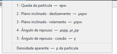
The Calibration menu opens wizards that automate the canonical tests: each one builds the case, runs the solver repeatedly while varying the target parameter, and writes the value it finds back into the material. The tests are numbered in the order they must be run — each starts from the parameters the previous ones have already fixed, and calibrating out of order propagates error.
| # · WIZARD | CALIBRATED PARAMETER | DEPENDS ON |
|---|---|---|
| 1 · Particle drop | Particle–wall restitution e_pw | — |
| 2 · Inclined plane · sliding | Sliding friction μs_pw | e_pw |
| 3 · Inclined plane · rolling | Rolling friction μr_pw | e_pw, μs_pw |
| 4 · Angle of repose | Particle–particle frictions μs_pp and μr_pp | e_pw, μs_pw, μr_pw |
| 5 · Angle of repose · cohesion | Cohesion: k (SJKR) or γ (JKR) | the previous ones + μs_pp/μr_pp |
| Bulk density | Particle density ρ | — (independent) |
The wizard checks its prerequisites on opening. If an earlier test has not been run in this session it warns you and lets you enter the value manually rather than blocking — useful when you already have the parameter from a bench test or from an earlier session. The heap in the repose test, for instance, settles against the container wall: without consistent μs_pw and μr_pw, the measured angle carries the error of the particle–wall contact.
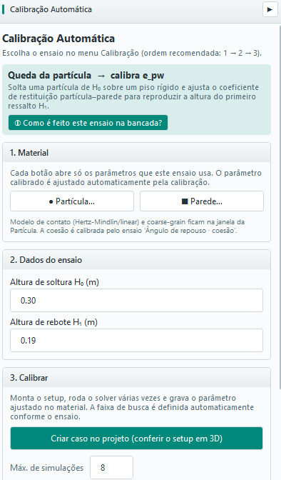
In the example shown, with a release height H₀ = 0.30 m and a rebound height H₁ = 0.19 m, the wizard estimates eₙ ≈ 0.796 for a spherical particle of radius 5 mm — consistent with equation 3.10 (√(0.19/0.30) ≈ 0.796). The wizard also lets you pick the contact model (Hertz–Mindlin or linear), coarse-graining (CGF), cohesion (JKR) and torsion (Marshall), plus buttons to edit the material and the wall of the test.
Configuring the test: what each block controls
Besides the target value measured on the bench, the panel exposes the variables of the test itself, grouped into blocks that appear according to the chosen protocol:
| BLOCK | WHAT IT CONTAINS |
|---|---|
| Test data | The bench-measured target: H₀/H₁ (drop), critical angle (inclined plane), angle of repose and heap base diameter, target density (bulk) |
| Test geometry | Diameter and height of the pouring cylinder in the repose test. 0 = automatic: diameter ≈ 20× the effective particle diameter and height 1.5× the diameter, the standard proportion in the literature |
| Cohesion | Heap calibration mode and cohesion model (Linear k or JKR γ) — test 5 only |
| Fixed parameters — inherited from the other tests | e_pp, e_pw, μs_pp, μr_pp, μs_pw, μr_pw that are not being adjusted in this test. They stay visible and editable rather than hidden |
| Reproduce the bench (experimental protocol) | Plane rotation rate (°/s), cylinder lift speed, pre-settling, filling and final settling times, and the friction of the tube itself. Unchecked, the test uses automatic quasi-static values |
| Optimiser | Number of iterations, angular tolerance (default 0.5°) and “Run until convergence” |
The Fixed parameters block is what makes the calibration auditable: in any test you can see exactly which values the remaining parameters are frozen at, and override them without leaving the screen. The Reproduce the bench block serves the opposite case: when the real test was not quasi-static — a plane raised quickly, a tube that was not smooth — and the simulation has to repeat those conditions for the comparison to mean anything.
Repose test modes and cohesion
The heap test (4 and 5) has a calibration mode that decides which parameters the optimiser moves, holding the rest fixed:
| MODE | ADJUSTS | WHEN TO USE |
|---|---|---|
| Dry | μs_pp + μr_pp | Non-cohesive material (test 4) |
| Cohesive — cohesion only | k or γ | p–p frictions already calibrated dry; only cohesion is left |
| Cohesive — μr_pp + cohesion | μr_pp + k/γ | The cohesive default: rolling and cohesion are the two that move the angle most |
| Cohesive advanced | μs_pp + μr_pp + k/γ | Wide search; more expensive and more prone to equivalent solutions (different sets giving the same angle) |
Cohesion is active only in the test where it is the parameter being sought — drop and inclined plane always run dry, so that adhesion does not contaminate e_pw and μs_pw. The dry tests still offer a Consider cohesion option among the fixed parameters, for when the material really is cohesive and ignoring that would distort the result.
How the angle of repose is measured
The reading is not a single straight line fitted across the heap. BrixDEM measures the flanks of the orthographic envelope over 8 azimuthal sectors and reports the robust mean across the valid directions. Three practical consequences:
- Only settled particles are counted — below a velocity threshold that scales with √(g·d). Strays still rolling used to stretch the apparent base and flatten the measured angle;
- The measurement is the average of the last few snapshots, which cuts the run-to-run noise without lengthening the test;
- The standard deviation across the 8 sectors is reported alongside. It measures heap asymmetry: a high spread means the heap is not axisymmetric and that result needs closer examination.
Why the angle may not rise when μ_r rises
It is natural to expect that increasing μ_r always raises the heap angle. However, CDT does not guarantee that the macroscopic angle grows monotonically with μ_r. The resisting torque is proportional to:
 (18.1)
but it acts only while relative rolling exists. With μs = 0.2, raising μ_r substantially can make the motion migrate from rolling to sliding. From that point on, what limits the inclination is mainly the sliding friction μs. Different avalanches and the formation of a flatter top may also occur, making one realisation end up slightly below the previous one.
18.6 Validating the model against reference experiments
Define the observable, measurement uncertainty and acceptance criterion before fitting the model. Use conditions held out from calibration to assess predictive ability. A tolerance selected for one case is not a universal DEM guarantee.
| Test | Observable | Consistent comparison |
|---|---|---|
| Angle of repose | Final angle and pile shape | Same apparatus, discharge method and region used to fit the slope. |
| Bulk density | Settled bed mass/volume | Same filled volume and settling protocol; exclude empty space outside the bed. |
| Inclined plane | Onset-of-motion angle | Distinguish sliding from rolling; tan θ ≈ μ applies to the matching sliding condition. |
| Normal rebound | e = |vout/vin| or √(h₂/h₁) | Same reference heights and surface; separate rotation, oblique impacts and air dissipation. |
| Hopper discharge | Mass flow rate and flow pattern | Same PSD, filling, outlet opening and rate calculation interval. |
| Rotating drum | Dynamic angle, regime and power/torque | Same fill level, speed and time window after startup. |
Bulk density and solids fraction
For occupied bed volume Vbed, calculate ρbulk = M/Vbed. For one solid density ρs, φs = ρbulk/ρs. Global φ in quick plots uses domain volume as denominator; it is not automatically bed solids fraction. Use a region consistent with the experiment; for clumps, check the union volume rather than double-counting overlapping pebbles. A change in φ can have different causes, including PSD, shape, filling procedure and friction.
Simulation–experiment comparison workflow
- Calibrate using the chosen tests (18.4–18.5), recording which data were used.
- Hold out validation conditions and reproduce geometry, materials and boundaries.
- Use the same observable definition and time window/sampling in the experiment and CSV.
- Calculate absolute deviation and, for nonzero references, relative error |simulation−reference|/|reference|.
- Compare against experimental uncertainty and the predefined criterion. If these data are then used for refitting, they become calibration data; hold out another condition for validation.
Calibrating and validating breakage against a reference test
Use a test protocol consistent with the source of the Ab-T10/PRM parameters. A DWT should record body mass and size, impactor/support geometry and stiffness, drop height or velocity, nominal energy, energy actually assigned to the event and fragment sieving. For Ab-t10, record breakage probability and t10 separately: t10 is the mass percentage passing one tenth of initial size.
- Prepare data: use samples of the actual ore, documenting preparation, shape, surface moisture and size range. Keep the same energy basis in experiment, fitting and simulation; mgh/m does not automatically equal absorbed work per mass.
- Calibrate: fit strength/selection at several energies and sizes. Then fit t10 and progeny size distribution to sieve data. Presets in 10.10 are documented starting points; choosing copper, coal or another material does not reproduce your sample or the published experiment.
- Build the virtual test: reproduce the body, support, impactor and initial conditions. Keep Young’s modulus and walls consistent with calibration and select a timestep that resolves fragments (12.6). Check mass, energy and isolated-body response before enlarging the case.
- Validate against reserved data: compare probability, t10 and cumulative PSD at sizes and energies not used in fitting. Report replica count, scatter and differences as well as the mean curve. A single preview curve or event does not establish validation.
- Check sensitivity: reduce Δt and refine fragment resolution, then repeat the quantities of interest. Only then examine the full process and any CGF changes.
Use ore references in the model for which they were fitted: parameters from a different DWT or JK selection model are not interchangeable with Ab-t10 S. For values, reproduction inputs and measured solver verification results, see Appendix H; for bibliographic provenance, see Appendix F.
Validating wet material
Begin with force and rupture verification between simple surfaces without breakage, as in Appendix H. Then compare wet material with independent flow, pile or shear experiments, measuring surface content, surface tension and contact angle under the test conditions. Check free/film, bridge and total liquid inventory and compare with the dry case. Agreement with a force correlation and conserved inventory verifies implementation but does not itself validate the material’s macroscopic response. Observe combination limits in 28.7.