
Tutorial 3 — Bucket elevator
Case recorded on video: geometry imported as STL, Elevator motion with reference drums, inlet at the boot, outlet at the discharge and diagnosis of the transport direction.
This tutorial reproduces the Elevador T3 case from the tutorial video. It is the most advanced motion case in the guide: the bucket receives the Elevator motion (Chapter 7.5), which replicates copies along a closed circuit between two drums — going up one side, rounding the upper drum and coming down the other. The tutorial also shows a real diagnostic workflow: the first run reveals the reversed transport direction, fixed by the sign of the velocity.
23.1 Case overview
| ITEM | VALUE USED |
|---|---|
| Geometry | 3 imported STLs: casing, bucket (copo) and drums |
| Motion | Elevator on the bucket, via Quick setup with two reference cylinders (radius 0.26 m); signed linear speed 0.5 m/s |
| Materials | Dedicated particle material (very low elastic modulus); walls with the Wall material |
| Insertion | Box inlet at the elevator boot; box outlet at the top discharge region |
| Coarse-graining | CGF = 4, preserving the time step (applied after the first test run) |
| Setup | Automatic Δt (Rayleigh), adaptive saving; 3 s verification run |
| Result | Buckets capture the material at the boot, climb the correct side and discharge at the top |
23.2 How the Elevator motion works
Before the step-by-step procedure, it is worth understanding what the Elevator motion does — it is what sets this case apart from every other in the guide. The Elevator turns a single STL (the bucket) into a set of copies that travel a closed circuit: two straight sections (up and down) joined by two semicircular arcs around the lower and upper drums — exactly the trajectory of an elevator belt. The bucket is not "dragged" by physics: the kinematics are prescribed (like every surface motion, Chapter 7.5), but the buckets exert forces and torques on the particles they touch — they capture material at the boot, carry it up and dump it at the discharge.
The path is defined by three geometric inputs and the behaviour of the assembly by four more parameters:
| FIELD | WHAT IT DEFINES |
|---|---|
| Drum center A / B (m) | The two circuit centers — lower and upper drums. Their distance defines the straight sections |
| Common drum axis | The vector of the axis around which the arcs are traced (the drum axis, e.g. Z) |
| Pitch radius (m) | The radius of the semicircular arcs — the distance from the drum center to the belt line |
| Signed linear speed (m/s) | Magnitude AND direction of travel along the circuit. The sign decides which side the buckets go up |
| Number of copies | How many buckets are evenly distributed along the path (2 to 200) |
| Initial set phase (0 to 1) | Shifts all buckets along the circuit — 0.5 advances half a lap |
| Local STL attachment point (m) | Which point of the bucket is "pinned" to the circuit line |
There are also two orientation options: Follow path while preserving initial orientation (the bucket goes up, around and down always "mouth up" — the mode used in the video and the correct one for buckets) and Follow conveyor tangent (the part rotates following the path direction — in that mode, local X is the travel, local Y the outward radial and local Z the drum axis). The current orientation of copy 1 is used as reference and the others follow the path relative to it.
All of this can be typed manually in the Advanced — edit path manually expander. But the practical route is the Quick setup: you create two reference cylinders (surfaces) at the drums, and the software extracts the centers, the axis and the pitch radius from them automatically — the workflow used in the video and detailed in Step 3.
23.3 Step by step
Step 1 — Import the elevator STLs
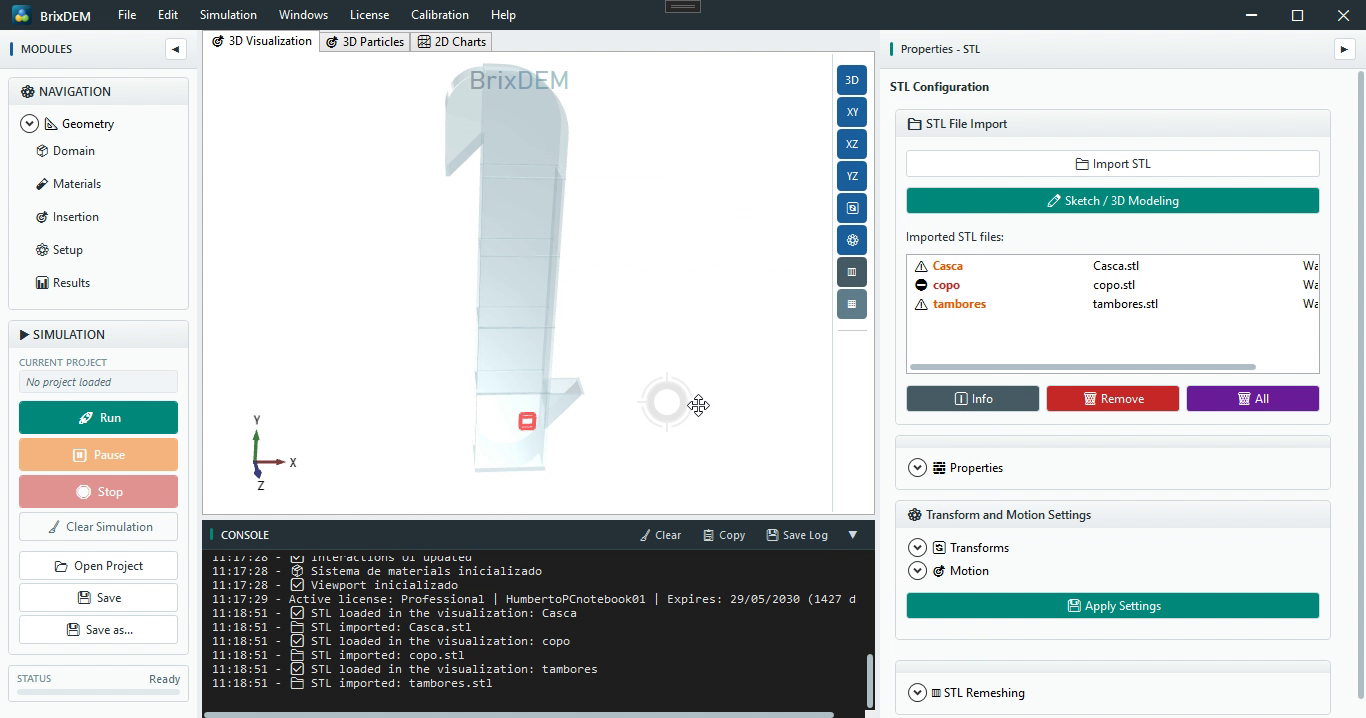
In Geometry › STL, import the three equipment files — Casca.stl (outer casing with the feed and discharge regions), copo.stl (a single bucket — the Elevator will replicate the rest) and tambores.stl (drums and belt, a visual/structural body only). The format can be ASCII or binary STL. Adjust the opacity of the casing and drums to see the interior of the equipment.
Then assign the wall material (Wall) to each of the three bodies and click Apply Properties body by body. On the bucket, also enable force and torque measurement — it lets you track the load on the buckets. Wear is not used in this case.
Step 2 — Create the drum reference cylinders
For the Quick setup, create in Geometry › Surfaces two cylinders that represent the circuit drums:
- Type = Cylinder, with the two axis points passing through the lower drum center (cylinder 1) and the upper drum center (cylinder 2), both with the axis along Z — the physical drum axis;
- Radius = 0.26 m — this value becomes the circuit pitch radius, so it must be the effective belt radius at the drum, not the outer pulley radius;
- Closed solid (with caps), Stationary motion and Wall material;
- Click Add Surface for each one (
cylinder01andcylinder02).
Step 3 — Configure the Elevator motion on the bucket
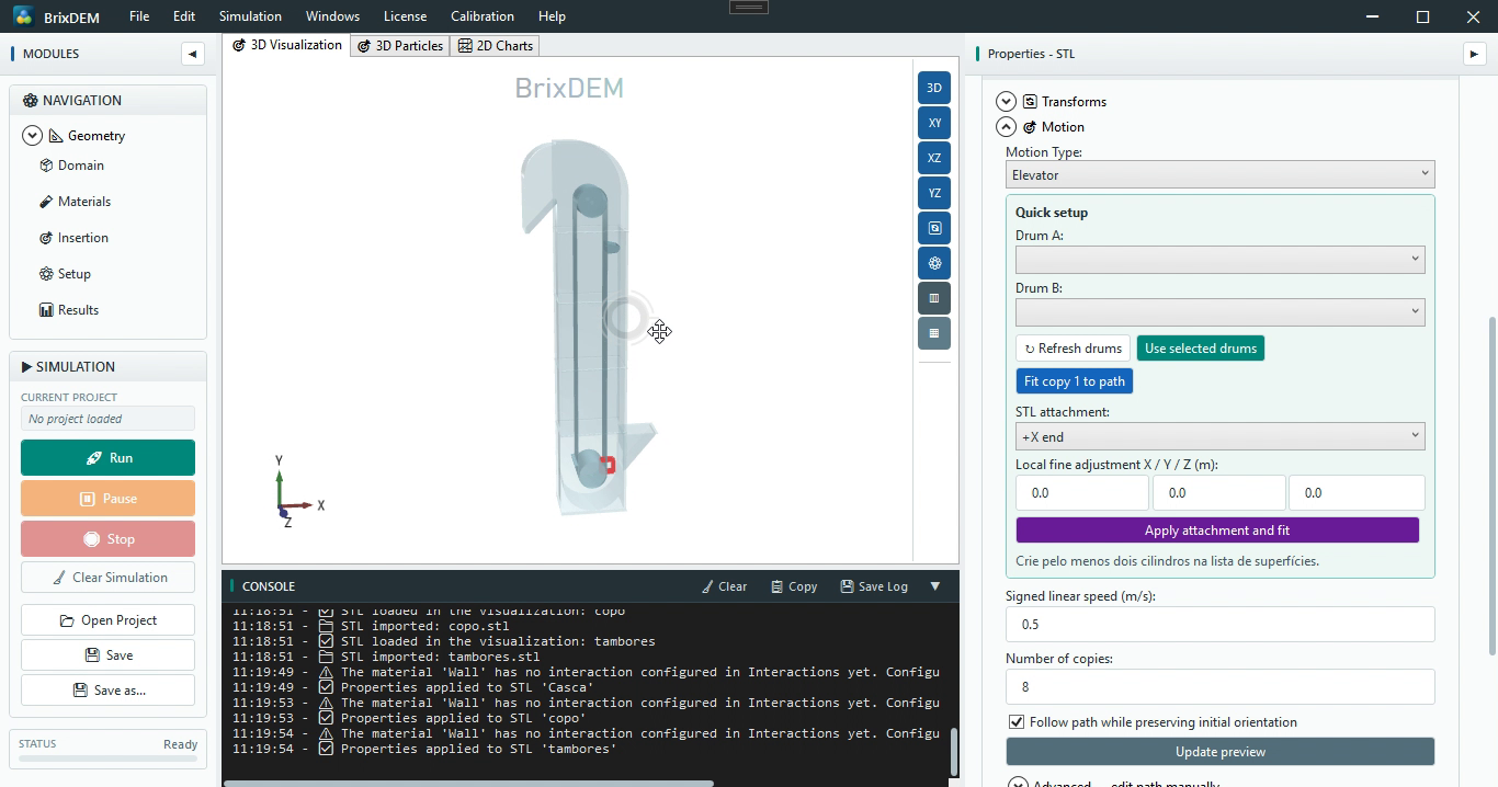
Select the bucket STL (copo) and, under Motion, choose Motion Type = Elevator. Follow the Quick setup panel sequence:
- ↻ Refresh drums — the software scans the surfaces and lists the available cylinders; select
cylinder01as Drum A andcylinder02as Drum B; - Use selected drums — the centers, the common axis and the pitch radius are extracted from the cylinders and filled into the path automatically;
- STL attachment — choose which point of the bucket is pinned to the circuit line: Center or one of the ends (−X/+X, −Y/+Y, −Z/+Z). In the video, the attachment used is the +X end — the back of the bucket faces the belt;
- Fit copy 1 to path — places the bucket on the computed trajectory;
- Local fine adjustment X / Y / Z — if the bucket does not sit exactly where it should, correct with small +/− increments and use Apply attachment and fit until the position is right (in the video this adjustment is iterative: "center, apply… more, less… done");
- Signed linear speed = 0.5 m/s and the desired number of copies — the buckets are evenly distributed along the circuit;
- Keep Follow path while preserving initial orientation checked — buckets must not rotate during the transport;
- Update preview and, finally, Apply on the body — the console confirms the transform.
Step 4 — Domain, material and interactions
In Domain, use Fit to Geometry to wrap the whole elevator — including the top, where the buckets round the upper drum. Create the particle material (Material1) with a very low elastic modulus — the elevator flow is dominated by gravity and by the bucket kinematics, but reducing stiffness can alter deformation and contacts; compare overlap, flow rate and power with a stiffer reference case (10.7 and 19.8) — and configure the two interactions: Material1 ↔ Material1 and Material1 ↔ Wall, saving each one.
Step 5 — Inlet at the boot and outlet at the top
Enable the geometry edge display (feature edges) — the casing becomes a line outline and the internal regions are visible to position the boxes precisely. Then:
- Inlet: Category = Inlet, Format = Box, material Material1. Place the box at the feed region (the elevator boot, where the buckets pass underneath and capture material), with downward injection velocity (0; −0.5; 0) and rate in particles per second. Use the 3D Edit Mode to drag the box to the feed mouth and click Add;
- Outlet: Category = Outlet, Format = Box — a box, not a plane, as stressed in the video: the box wraps the whole top discharge region, and any particle entering it is removed from the simulation, representing the material that left through the discharge duct. Leave an additional margin along the launch direction to also capture the particles hurled farther.
Step 6 — Setup, save and run
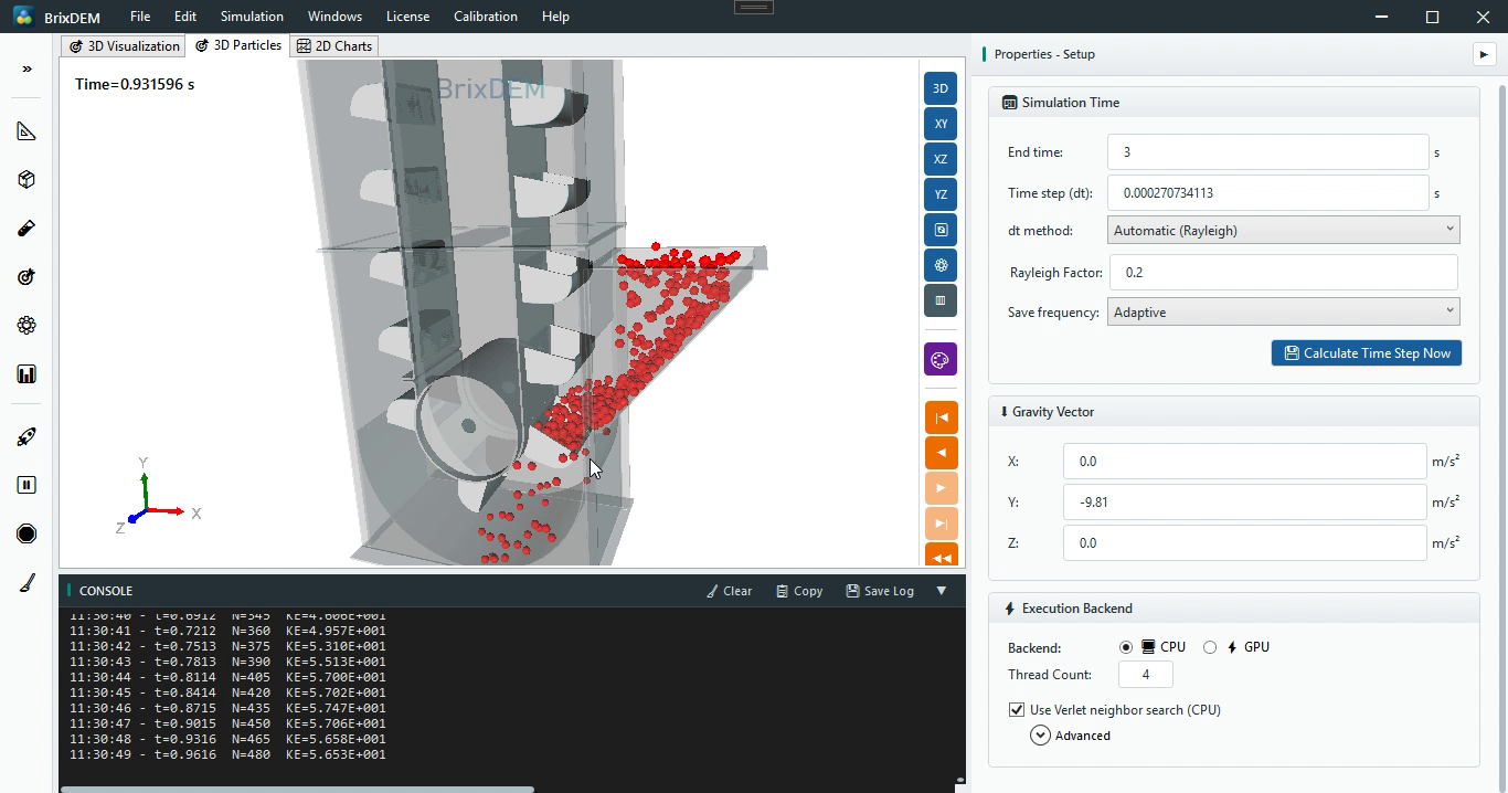
In Setup: automatic Δt (Rayleigh) with factor 0.2, adaptive saving and the desired backend/threads (CPU or GPU). Save the project (in the video, Elevador_Tutorial01) and run, following it in the 3D Particles tab — watch the three phases: capture at the boot, ascending transport and discharge at the top.
Step 7 — Diagnose and fix the transport direction
In the first run of the video, two problems show up — and the fix workflow is the most instructive part of the case:
- The buckets go up the wrong side — material is captured but transported in the reverse direction. The cause is the sign of the signed linear speed: invert it (0.5 → −0.5, or vice versa) in the Elevator panel and click Apply. There is no need to touch the geometry or the drums;
- The particles are too small for the bucket — they visually disappear and the cost is high. The fix in the video: coarse-graining CGF = 4 preserving the time step, which multiplies the radius by 4 and cuts the count by 64 (Chapter 10.7).
After the two fixes, reduce the end time to 3 s and run a short verification, as in the video — the goal is just to confirm the scheme: particles enter, are captured and go up the right side. Once the direction is confirmed, extend the end time for the real study.
Step 8 — Scalars and charts
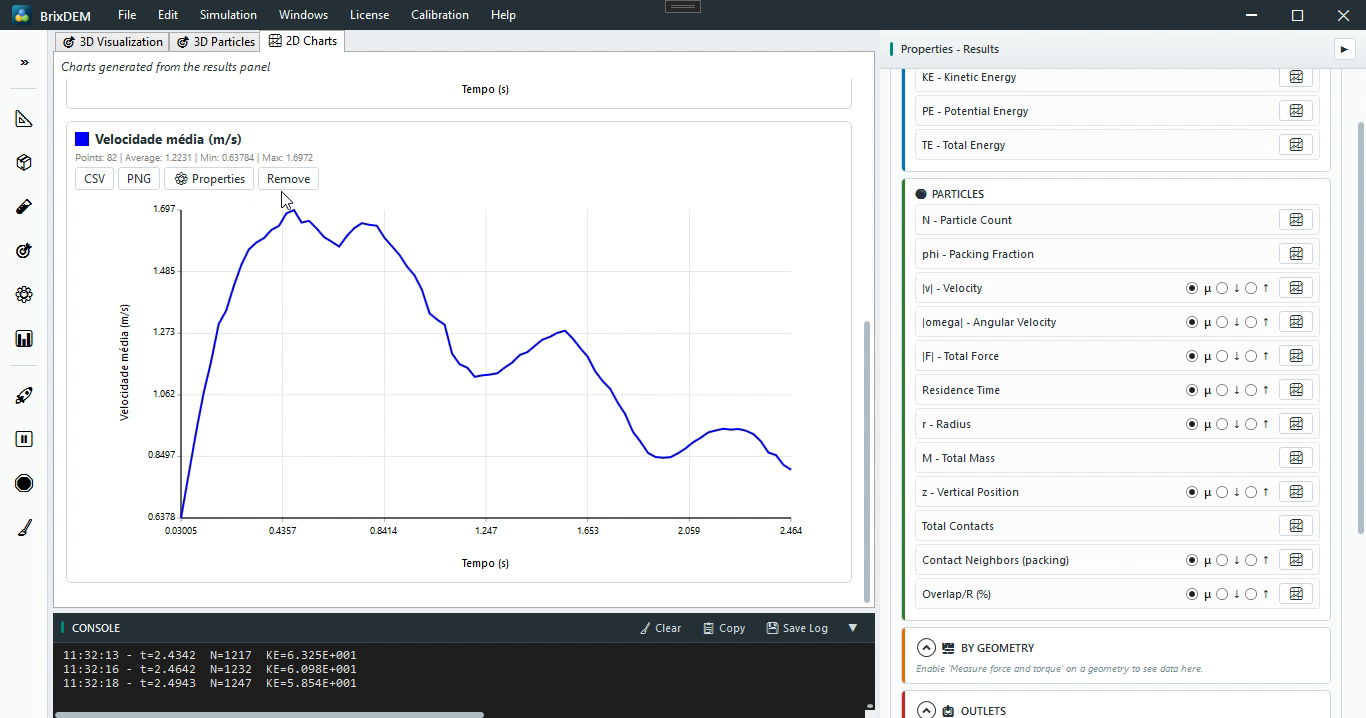
With the case running in the right direction, apply the velocity scalar limiting the colorbar range — the material climbing in the buckets stands out against the resting bed at the boot. In Results, the automatic charts complete the analysis:
| CHART | WHAT IT REVEALS IN THE ELEVATOR |
|---|---|
| KE — Kinetic energy | Regularity of the regime; periodic peaks follow the bucket passages |
| M — Total mass | Grows while the inlet feeds; the slope drops when discharge balances feeding |
| Outlet flow | Material effectively discharged at the top — the elevator capacity |
| Mean residence time | How long the material stays in the circuit (boot → bucket → discharge) |
| |v| — Mean velocity | Agitation level; correlates with the belt speed |
23.4 Interpreting the result
The elevator is a case where the prescribed kinematics (Elevator motion) dominates the result: capture at the boot, upward transport and discharge at the top depend on the direction, speed and spacing of the buckets. Growing total mass with stabilising outlet flow indicates balanced feeding and discharge; the mean residence time measures how long the material stays in the circuit.