
Tutorial 1 — Double-cone mixer
Complete case recorded on video: create the mixer in the Sketch Modeler, apply ramped rotation, fill with particles and analyse the mixing.
This tutorial reproduces, step by step, the Misturador T1 case demonstrated in the BrixDEM tutorial video. It is a simple, fast-running case that exercises the full cycle with a parametric geometry from the Sketch Modeler and a ramped rotational motion: the double cone is created internally, is rotated about the X axis, is instantly filled with particles and runs until the bed settles.
21.1 Case overview
| ITEM | VALUE USED |
|---|---|
| Geometry | Parametric double-cone mixer: body Ø 2.0 m, each cone 1.2 m, central band 0.4 m, nozzles Ø 0.4 m |
| Motion | Rotational, ω = (9; 0; 0) rad/s, center (0; 0; 0), velocity ramp (start 1.5 s; shutdown at 10 s) |
| Materials | Particle and wall with density 1000 kg/m³; interactions with default values + rolling friction |
| Inlet | Cylinder on the X axis from (−1; 0; 0) to (1; 0; 0), radius 0.45 m; 5000 particles, instant fill |
| Coarse-graining | CGF = 3, preserving the time scale |
| Setup | End time 15 s, automatic Δt (Rayleigh, factor 0.2), adaptive saving, CPU 4 threads + Verlet |
| Result | ≈ 1900 particles mixed in cascade; bed settled after the ramp ends |
21.2 Step by step
Step 1 — Create the double cone in the Sketch Modeler
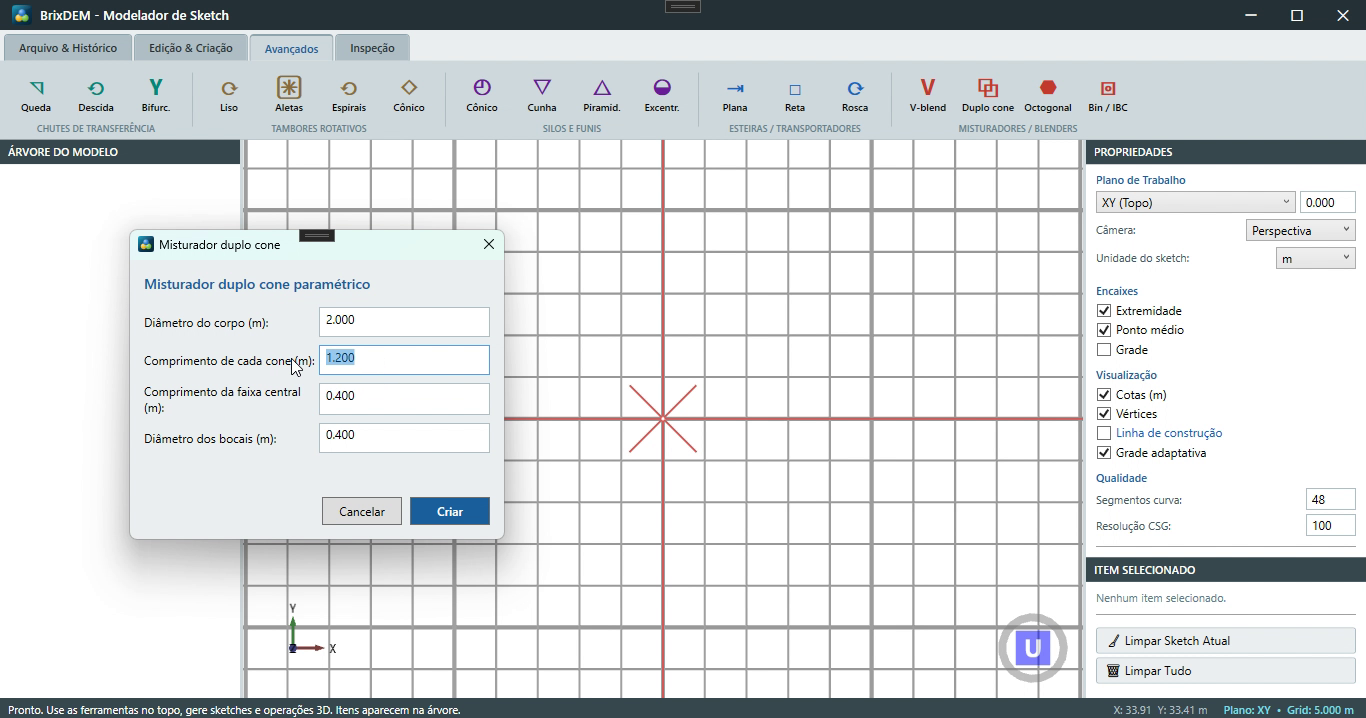
In the Geometry › STL panel, click Sketch / 3D Modeling and open the Advanced tab. There you find the ready-made equipment families — chutes, drums, silos, conveyors and mixers. Under Mixers / Blenders, click Double cone. The parametric form controls the whole equipment geometry:
| FIELD | VALUE IN THE VIDEO | WHAT IT CONTROLS |
|---|---|---|
| Body diameter | 2.0 m | Diameter of the central section; defines the working volume of the mixer |
| Length of each cone | 1.2 m | Height of each cone; longer cones = steeper walls |
| Central band length | 0.4 m | Cylindrical section between the two cones |
| Nozzle diameter | 0.4 m | Openings at the tips (loading/discharge in the real equipment) |
Fill in the values and click Create. Adjust the opacity in the Sketch if you want to inspect the interior. The solid appears in the model tree already centered at the origin, with the revolution axis along X — this matters in Step 2, because the rotation center can then be simply (0; 0; 0).
In the File & History tab, save the sketch in a tutorial folder (in the video: folder Misturador_Tutorial01, file "misturador sketch") — the parametric geometry can be reopened and edited later. Then use Send: the geometry enters the BrixDEM main window directly as an STL (MisturadorDuploCone1), with no intermediate file.
Step 2 — Prescribe the ramped rotational motion
With the STL selected in the Geometry › STL panel, open Transform and Motion Settings › Motion:
- Motion Type = Rotational — the body spins about a fixed axis and drags the granular bed;
- Angular velocity = (9; 0; 0) rad/s — the vector defines both the axis (X, the physical axis of the double cone) and the magnitude (9 rad/s ≈ 86 rpm). Remember: the unit is rad/s, not rpm (Chapter 7.5);
- Rotation Center = (0; 0; 0) — the spin axis passes through the origin, where the Sketch created the body. If the geometry were displaced, the center would have to follow the physical axis, otherwise the body "orbits" instead of spinning about itself.
Enable Use velocity ramp. The ramp avoids the numerical shock of an instantaneous start (the wall would "slam" into the resting particles) and lets you schedule the stop: in the video, the motion starts accelerating at ≈ 1.5 s, reaches full speed and is switched off at 10 s, decelerating to rest before the end of the simulation. Click Apply Settings — the console confirms the ramp and the applied transforms.
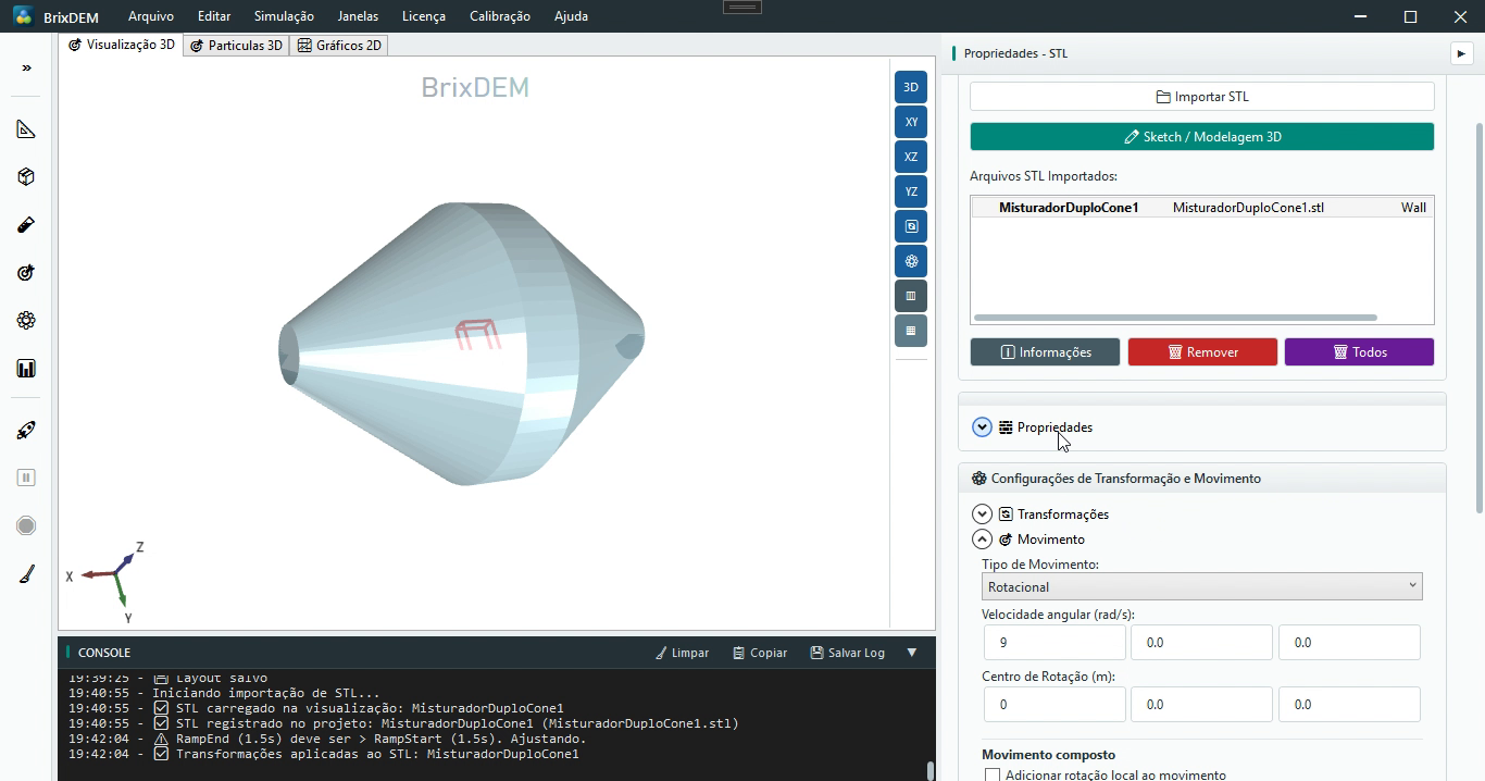
Still in the STL properties: confirm the wall material (Wall) and check Measure force and torque for this geometry — without it, body_forces.csv (body force, torque and power, Chapter 16.10) is not written. The Info button summarises the mesh (triangle count, dimensions), the transforms and whether wear/force are enabled. In the video some non-critical mesh warnings show up — they can be ignored; critical ones (open mesh, inverted normals) cannot.
Two visualisation controls worth knowing from here on: the body opacity (to see particles inside the closed geometry) and the option to keep the body in 3D only, in the simulation, or both.
Step 3 — Fit the domain
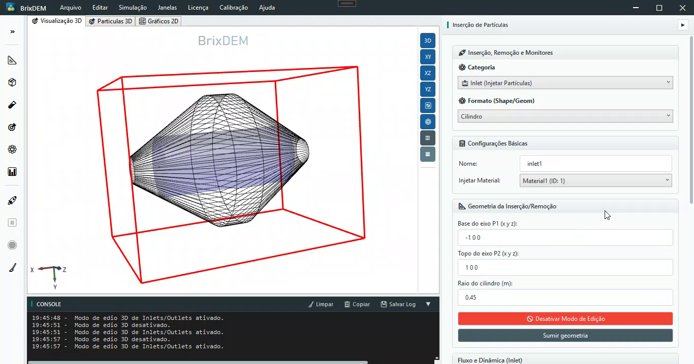
Open Domain and click Fit to Geometry: the domain (red box) is sized automatically around the STL with a margin — in the video, ≈ 3.2 × 2.4 × 2.4 m. Deletion of escaping particles depends on the removal option, margin and checking interval (9.5). For this enclosed mixer, check that the fitted domain contains the full material trajectory.
Step 4 — Materials, interactions and coarse-graining
In Materials, create the particle material with density 1000 kg/m³ and edit the wall material to the same density and Poisson values — light, soft materials keep this demo case fast. Then, in Interaction Configuration, define both contact pairs of this case:
- Particle ↔ Wall (Material1 ↔ Wall) — default restitution and friction, with rolling friction enabled;
- Particle ↔ Particle (Material1 ↔ Material1) — same default values.
Click Save Interaction for each pair. Without a defined interaction the solver does not know how to compute that pair's contact (Chapter 10.4). The same panel exposes cohesion (not used here) and coarse-graining: apply CGF = 3 — each simulated particle now represents ≈ 27 real ones (3³). Cost reduction is not necessarily proportional, and flow equivalence must be checked against CGF = 1; also check the E control and timestep (10.7).
Step 5 — Create the cylindrical inlet with instant fill
Open Insertion. Category = Inlet (Inject Particles), Format = Cylinder, and under Basic Settings select the particle material (Material1 — not Wall). The cylinder geometry is given by the two axis points and the radius:
- Axis base P1 = (−1; 0; 0) and Axis top P2 = (1; 0; 0) — the cylinder runs along the X axis, crossing the central region of the mixer;
- Radius = 0.45 m — in the video the radius was increased gradually (0.4 → 0.45) using the 3D Edit Mode until the cylinder filled the body well without touching the wall: particles must not be born in contact with the geometry.
In the Flow and Dynamics expander, set the injection direction to −Y (downwards), the quantity to 5000 particles and check Instant fill: instead of injecting at a rate, the whole cylinder is filled at once at the initial instant, forming the bed immediately. Click Add and confirm that inlet1 shows up under Configured Items.
Step 6 — Numerical setup
In Setup: End time = 15 s; dt method = Automatic (Rayleigh) with factor 0.2 — the solver computes the safe Δt from the smallest Rayleigh time of the materials (in the video Δt ≈ 3.4×10⁻⁴ s) and recomputes it via Calculate Time Step Now; Save frequency = Adaptive; gravity (0; −9.81; 0); and CPU backend with 4 threads with Verlet neighbor search enabled (Chapter 12.4).
Step 7 — Save and run
Save the project with Save as (in the video: Misturador01) — BrixDEM creates the simulation folder and generates the files — and click Run. Follow the console: at each interval it prints t=… N=… KE=… (physical time, particle count and kinetic energy). In the 3D Particles tab:
- 0 to ~1.5 s — the instant-fill particles fall and settle at the bottom (rotation has not started yet);
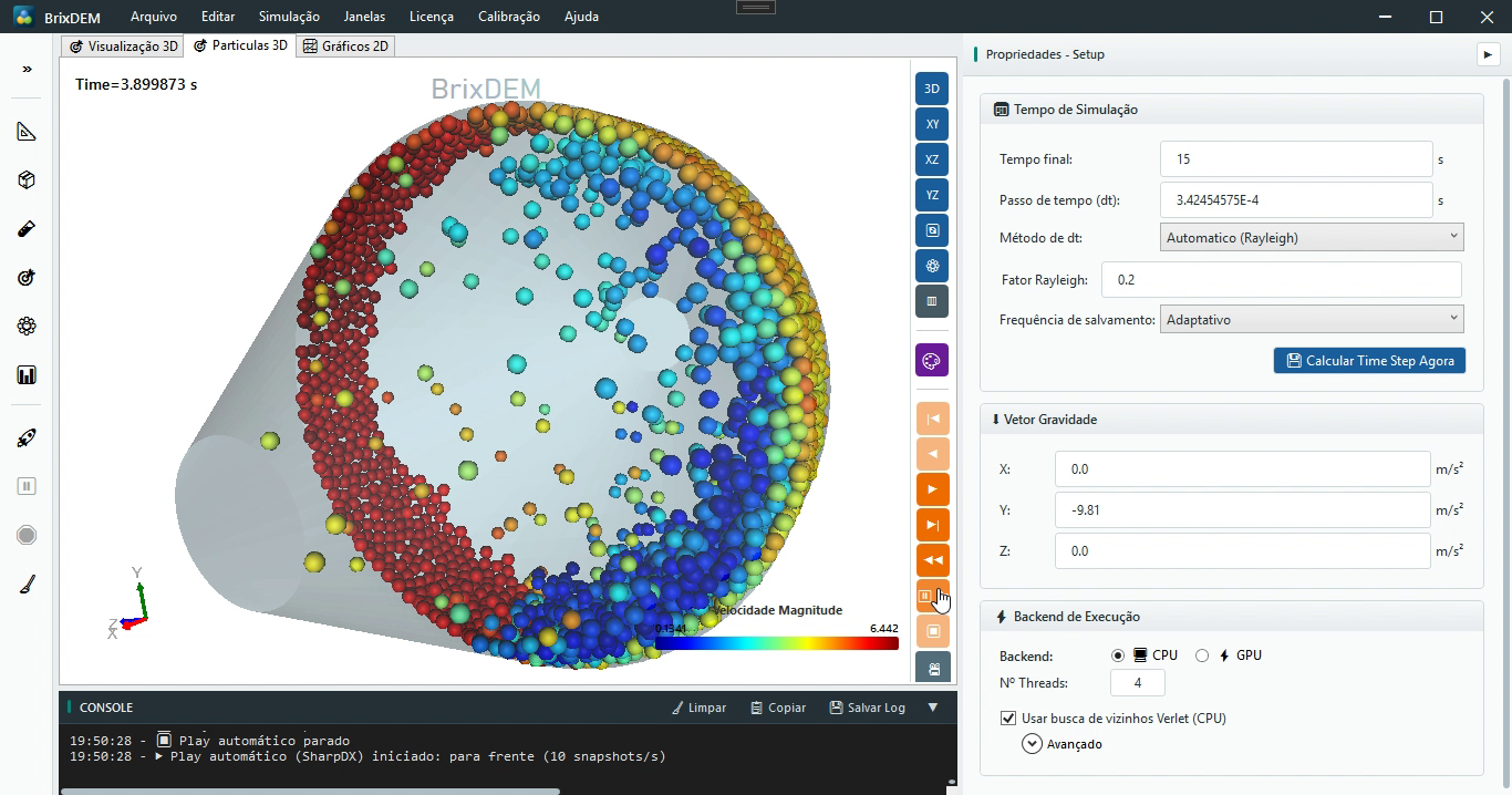
- ~1.5 to 10 s — the ramp accelerates the body up to 9 rad/s: the bed is dragged by the wall, climbs, and cascades down the free surface — the mixing mechanism of the double cone;
- 10 to 15 s — the motion decelerates and stops; the bed relaxes to rest.
Via the scalar button (palette icon), choose Variable = Velocity Magnitude and apply. Adjust the body opacity and the light direction in the scene settings to see the material inside the mixer, as done in the video.
21.3 Interpreting the result
Three main readings of this case:
- Particle count — ≈ 1862 of the 5000 requested were created: instant fill prevents overlaps between particles and with the wall, so only what fits in the cylinder volume with the coarse radius (CGF 3) is created. Not an error — it is the protection against the initial "explosion" (Chapter 11.5);
- Mean velocity curve — rises with the ramp, shows a peak in the cascade regime and decays to rest after the shutdown at 10 s. The chart reproduces the profile programmed in the motion ramp: the signature that the prescribed motion worked;
- Velocity field — in Figure 21.4, the fast ring (red) along the wall and the slow core (blue) show the shear gradient that drives mixing in the double cone.
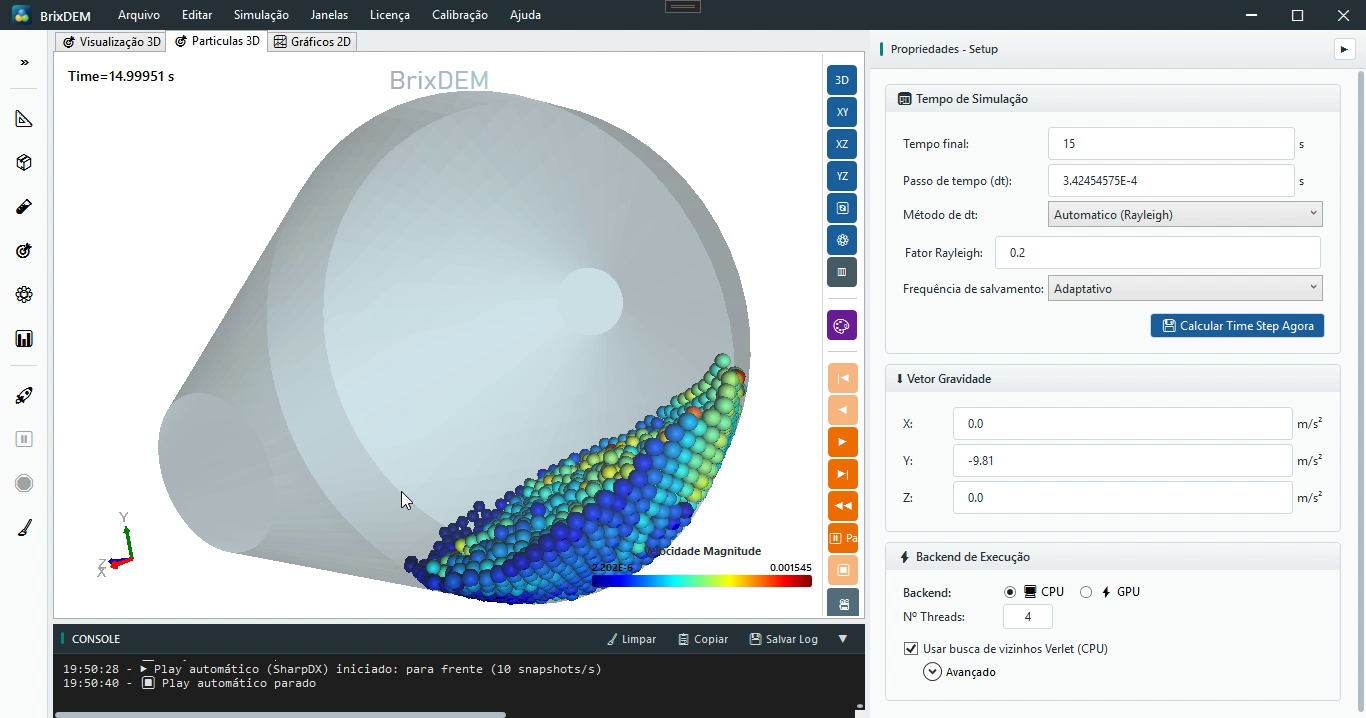
To document the case as in the video: step through the snapshots to the desired instant, position the camera, and use the video recording (Chapter 15.7) — choose codec/FPS in the visualisation properties and save; the file opens from its output folder when recording finishes.
21.4 Variations to try
- Rotation speed: increase or reduce ω to change the cascade regime and the mixing time;
- Two species: inject two materials (Chapter 11.7) and follow the Lacey index (Chapter 16.6) to quantify the mixing;
- Snapshot and video: position the camera, recreate the case and use video recording (Chapter 15.7) to document the result;
- CGF = 1: repeat without coarse-graining and compare the mixing pattern and the computational cost (Chapter 10.7).