
Analytical Verification of the Solver
Equation and implementation checks for contact, rigid bodies, clumps, liquid bridges and breakage. Each result states its reference, parameters and evidence limits.
1. Purpose and methodology
Verification establishes that the selected equations are solved correctly. Validation compares predictions with independent physical data; calibration fits parameters to a set of tests. This appendix collects numerical equation checks: plots compare analytical references and solver response. Parameters and procedures accompany each case; theoretical formulation is in Chapter 3. Agreement with a law does not establish experimental material validation.
For a nonzero reference, relative error = |measured−reference|/|reference|. Tables state whether errors are fractions or percentages; probability errors use percentage points (pp). For a zero reference, use the absolute residual with its unit. Results refer to each case’s stated conditions; reproduce the same parameters and observables.
2. Normal sphere–wall restitution
What this case verifies
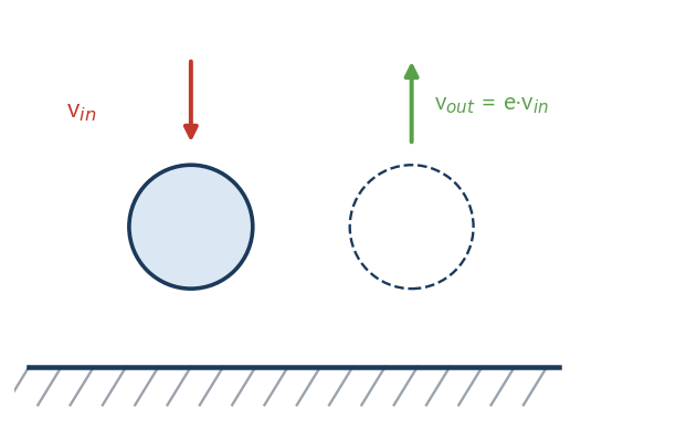
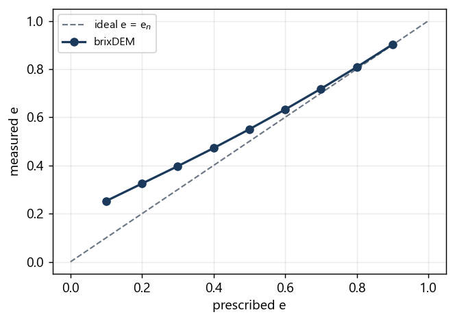
A sphere hits the wall head on, without friction and without gravity. The restitution coefficient e = |vout/vin| measures the fraction of speed preserved. It is the most basic test and covers, at once, the normal contact force, the damping, the prescribed restitution, the time integration and the approximate conservation of energy.
Parameters to reproduce it in the GUI
| Panel / field | Value |
|---|---|
| Material · Radius | 0.005 m |
| Material · Density | 2500 kg/m³ |
| Material · Young's modulus (E) | 1×10⁷ Pa |
| Material · Poisson (ν) | 0.30 |
| Material · Restitution (e) | 0.1 to 0.9 (swept) |
| Material · Friction (μ) | 0 |
| Contact interaction | Hertz–Mindlin |
| Setup · Gravity / Δt | (0,0,0) / 1×10⁻⁶ s |
| Initial condition | v = (0, −1, 0) m/s above the floor |
Result
| Quantity | Analytical | brixDEM | Error [%] |
|---|---|---|---|
| e = 0.10 | 0.10 | 0.2526 | 152.6 |
| e = 0.20 | 0.20 | 0.3248 | 62.4 |
| e = 0.30 | 0.30 | 0.3971 | 32.4 |
| e = 0.40 | 0.40 | 0.4720 | 18.0 |
| e = 0.50 | 0.50 | 0.5503 | 10.1 |
| e = 0.60 | 0.60 | 0.6323 | 5.4 |
| e = 0.70 | 0.70 | 0.7182 | 2.6 |
| e = 0.80 | 0.80 | 0.8081 | 1.0 |
| e = 0.90 | 0.90 | 0.9020 | 0.2 |
3. Oblique collision with friction
What this case verifies
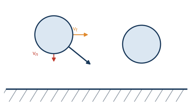
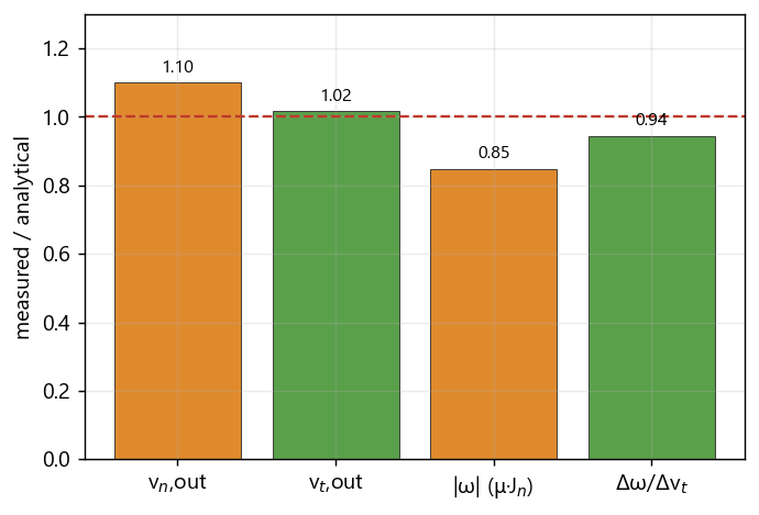
The sphere hits the wall with normal and tangential velocity components and no initial spin. Friction converts part of the linear momentum into rotation. The core test is the coupling between the change in tangential velocity and the change in rotation, where sign or magnitude errors of the torque would show up.
Parameters to reproduce it in the GUI
| Panel / field | Value |
|---|---|
| Material · Radius / Density | 0.005 m / 2500 kg/m³ |
| Material · Young / Poisson | 1×10⁷ Pa / 0.30 |
| Material · Restitution (e) | 0.5 |
| Material · Friction (μ) | 0.10 |
| Contact interaction | Hertz–Mindlin |
| Setup · Gravity / Δt | (0,0,0) / 1×10⁻⁶ s |
| Initial condition | v = (1, −1, 0) m/s, ω = 0 |
Result
| Quantity | Analytical | brixDEM | Error [%] |
|---|---|---|---|
| Coupling Δω/Δv_t [1/m] | 500.0 | 472.4 | 5.5 (OK) |
| v_n,out [m/s] | 0.500 | 0.550 | 10.1 (model) |
| v_t,out [m/s] | 0.850 | 0.865 | 1.8 (OK) |
| |ω| vs μ·J_n [rad/s] | 75.0 | 63.7 | 15.1 (model) |
4. Sliding into pure rolling
What this case verifies
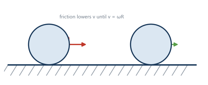
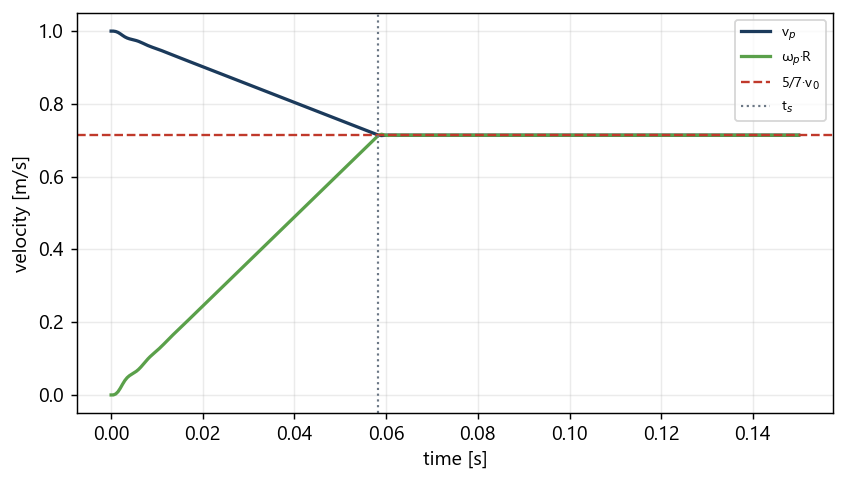
A sphere is launched with horizontal velocity v₀ on a floor with friction, without initial spin. Friction decelerates it and spins it up at the same time, until pure rolling (v = ω·R) sets in and the velocities become constant. It verifies Coulomb friction, torque, moment of inertia and the regime transition.
Parameters to reproduce it in the GUI
| Panel / field | Value |
|---|---|
| Material · Radius / Density | 0.005 m / 2500 kg/m³ |
| Material · Young / Poisson | 1×10⁷ Pa / 0.30 |
| Material · Friction (μ) | 0.5 |
| Material · Rolling resistance | None |
| Contact interaction | Hertz–Mindlin |
| Setup · Gravity / Δt | (0, −9.81, 0) / 2×10⁻⁶ s |
| Initial condition | v = (1, 0, 0) m/s, ω = 0, on the floor |
Result
| Quantity | Analytical | brixDEM | Error [%] |
|---|---|---|---|
| v_f [m/s] | 0.71429 | 0.71394 | 0.05 |
| ω_f [rad/s] | 142.857 | 142.79 | 0.05 |
| t_s [s] | 0.05827 | ≈0.058 | < 1 |
5. Sphere on an inclined plane
What this case verifies
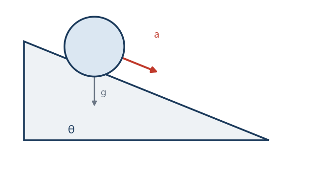
On a ramp the sphere has two regimes. With enough friction it rolls without sliding and the acceleration is a = (5/7)·g·sinθ. With low friction it slides and a = g(sinθ − μ·cosθ). Verifying both separately confirms that the solver tells the regimes apart and combines gravity, rotation and contact.
Result
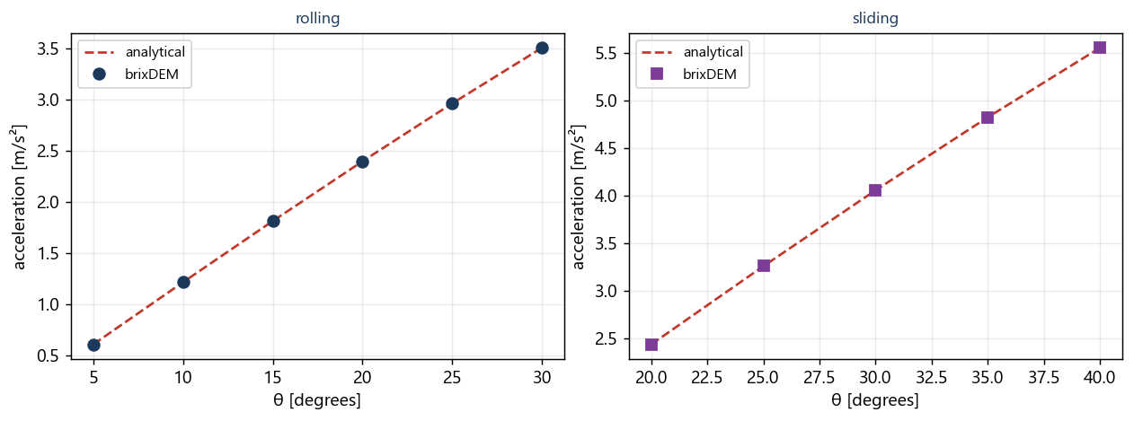
Case 4, rolling without sliding (μ = 0.6):
| θ [°] | a analytical [m/s²] | a brixDEM [m/s²] | error [%] |
|---|---|---|---|
| 5 | 0.6107 | 0.6104 | 0.05 |
| 10 | 1.2168 | 1.2162 | 0.05 |
| 15 | 1.8136 | 1.8127 | 0.05 |
| 20 | 2.3966 | 2.3955 | 0.05 |
| 25 | 2.9613 | 2.9600 | 0.05 |
| 30 | 3.5036 | 3.5020 | 0.04 |
Case 5, sliding (μ = 0.10):
| θ [°] | a analytical [m/s²] | a brixDEM [m/s²] | error [%] |
|---|---|---|---|
| 20 | 2.4334 | 2.4334 | 0.00 |
| 25 | 3.2568 | 3.2568 | 0.00 |
| 30 | 4.0554 | 4.0554 | 0.00 |
| 35 | 4.8232 | 4.8232 | 0.00 |
| 40 | 5.5543 | 5.5543 | 0.00 |
6. Rolling threshold (rolling resistance)
What this case verifies
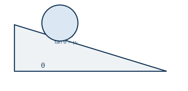
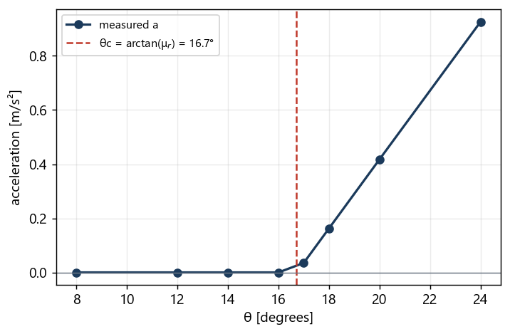
With rolling resistance active (CDT model, μr = 0.3) and high friction to prevent sliding, the sphere only starts rolling when the inclination exceeds θc = arctan(μr). Below that it stays static. It verifies the direction and the threshold of the rolling resistance torque.
Parameters to reproduce it in the GUI
| Panel / field | Value |
|---|---|
| Material · Friction (μ) | 0.60 (prevents sliding) |
| Material · Rolling resistance | CDT, μ_r = 0.30 |
| Contact interaction | Hertz–Mindlin |
| Geometry | Plane inclined by θ (swept 8° to 24°) |
| Setup · Gravity / Δt | (0,−9.81,0) / 2×10⁻⁶ s |
| Initial condition | at rest on the ramp |
Result
| θ [°] | Reported acceleration [m/s²] | State |
|---|---|---|
| 8 | 0.0000 | static |
| 12 | -0.0000 | static |
| 14 | 0.0000 | static |
| 16 | -0.0000 | static |
| 17 | 0.0351 | rolling |
| 18 | 0.1627 | rolling |
| 20 | 0.4178 | rolling |
| 24 | 0.9262 | rolling |
7. Braking by rolling resistance
What this case verifies
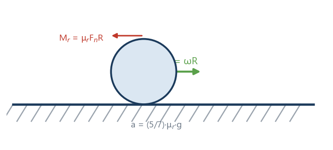
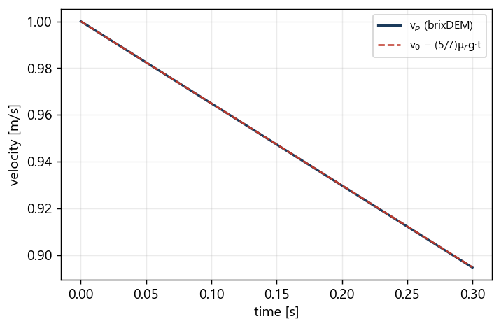
A sphere in pure rolling on a horizontal floor, with rolling resistance (CDT, μr = 0.05), decelerates linearly until it stops. It verifies the magnitude of the deceleration imposed by the rolling torque. The correct value for this model is (5/7)·μr·g, obtained from the angular momentum balance at the contact point; the simplified form (2/5)·μr·g does not correspond to this model.
Parameters to reproduce it in the GUI
| Panel / field | Value |
|---|---|
| Material · Friction (μ) | 0.5 |
| Material · Rolling resistance | CDT, μ_r = 0.05 |
| Contact interaction | Hertz–Mindlin |
| Setup · Gravity / Δt | (0,−9.81,0) / 2×10⁻⁶ s |
| Initial condition | pure rolling: v=(1,0,0), ω_z=−v/R |
Result
| Quantity | Analytical | brixDEM | Error [%] |
|---|---|---|---|
| deceleration a [m/s²] | −0.3504 | −0.3508 | 0.1 |
8. JKR adhesion between two spheres
What this case verifies
Two cohesive spheres (JKR model) are slowly pulled apart; the largest tensile force before rupture (snap-off) is measured. It verifies the sign and magnitude of the adhesion and the separation criterion. JKR cohesion keeps the bonded state from first touch and sustains tension across an already open gap until it breaks at pull-off — behavior that holds for the particle-to-particle pair and for wall contact alike (Case 8b).
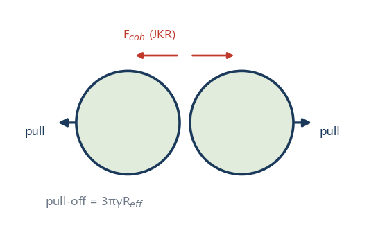
Parameters to reproduce it in the GUI
| Panel / field | Value |
|---|---|
| Material · Radius / Density | 0.005 m / 2500 kg/m³ |
| Material · Young | 1×10⁷ Pa |
| Material · Cohesion | JKR |
| Material · Surface energy (γ) | 0.10 J/m² |
| Contact interaction | Hertz–Mindlin + JKR |
| Setup · Gravity / Δt | (0,0,0) / 5×10⁻⁷ s |
| Initial condition | two spheres in contact, separating slowly |
Result
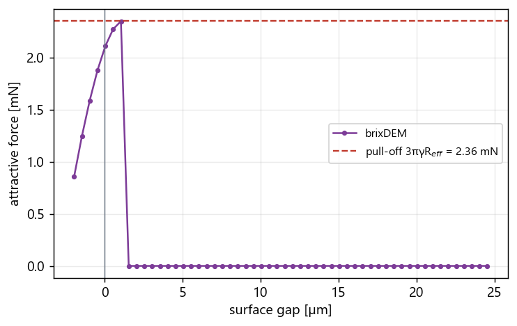
| Quantity | Analytical | brixDEM | Error [%] |
|---|---|---|---|
| F_pull-off [mN] | 2.3562 | 2.3536 | 0.11 |
Extension: JKR adhesion at a wall (Case 8b)
The same pair from Case 8 was repeated replacing one sphere with a flat wall carrying JKR cohesion and the same γ. The wall model uses the full JKR normal force: it keeps the bonded state during separation and breaks at the analytical snap-off, exactly like the particle-to-particle pair. The only difference is the effective radius — R_eff = R/2 between two equal spheres, R_eff = R against the flat wall — which doubles the pull-off force for the same γ.
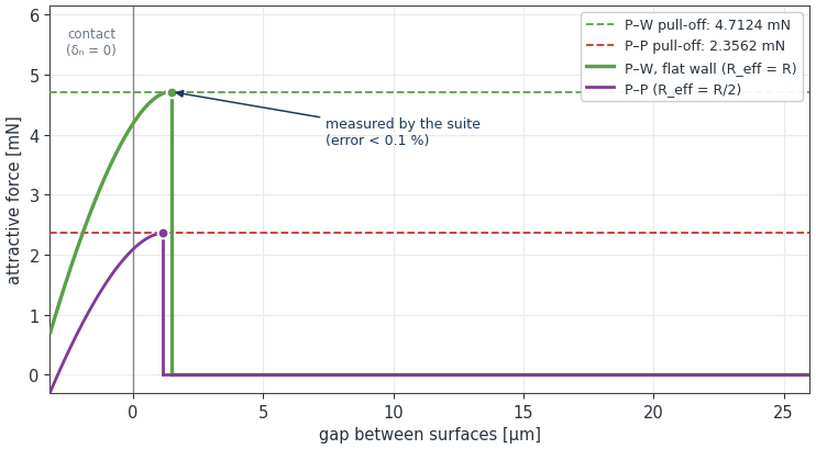
Result
| Quantity | Analytical | brixDEM | Error |
|---|---|---|---|
| Particle–wall F_pull | 4.7124 mN | 4.7124 mN | < 0.01 % |
| Particle–wall rupture gap | 1.4526 µm | 1.4513 µm | 0.09 % |
| Particle–wall F(δ) curve | analytical solution | max relative error 4.19×10⁻⁶ | — |
| Particle–particle F_pull (reference) | 2.3562 mN | 2.3562 mN | < 0.01 % |
| Particle–particle rupture gap | 1.1529 µm | 1.1521 µm | 0.07 % |
9. Free-body 6-DOF: torque-free rotation and DEM coupling
What this case verifies
The Free-body 6-DOF mode (Chapter 7.11) has two independent halves, and this appendix covers both. The first is the integrator: torque-free rotation of a body with three distinct principal moments, which only comes out right if the gyroscopic term ω × (I ω) exists and the quaternion is normalized. The second is the coupling: transmission of force and torque from the contact point to the center of mass, and the corresponding reaction on the particle.
Part A — torque-free rotation (Dzhanibekov effect)
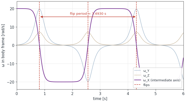
A body spinning about the intermediate axis sits in unstable equilibrium and must flip periodically, with a closed-form period — the tennis racket theorem. Since the case uses no particles, a failure points straight at the integrator, never at the contact model.
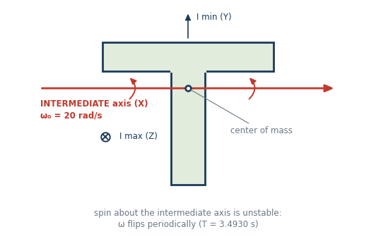
| Panel / field | Value |
|---|---|
| Body · geometry / density | T-handle: bar 120 × 20 mm, stem 24 × 80 mm, thickness 20 mm, recentred on the center of mass / 2650 kg/m³ |
| Body · Mass and inertia | 0.228960 kg; Ixx = 2.074773×10⁻⁴; Iyy = 1.651565×10⁻⁴; Izz = 3.573698×10⁻⁴ kg·m² |
| Body · Motion type | Free-body 6-DOF, preset Free — 6 degrees of freedom; quaternion 1,0,0,0; no lock, spring or limit |
| Body · Initial angular velocity | ω = (20.00; 0.10; 0.10) rad/s — without the 0.10 perturbation on the other two axes the body stays in unstable equilibrium and never flips |
| Setup · Gravity / Δt / duration | (0,0,0) / ≤ 1×10⁻⁵ s / 6 s, no particles and no contact |
| Quantity | Reference value | Tolerance |
|---|---|---|
| \|L\| in world frame | 4.149733418×10⁻³ kg·m²/s | relative drift < 1×10⁻⁴ over 6 s |
| Rotational energy | 4.149807930×10⁻² J | relative drift < 1×10⁻⁴ over 6 s |
| Flip period | 3.4930 s (zeros at 0.8156 / 2.5621 / 4.3086 s) | 2 % |
Part B — DEM coupling (measured)
The coupling is covered by 25 free-body checks — gravity and quaternion normalization, full inertia tensor, locks and limits, simultaneous STL contacts (n = 2, 3 and 8), persistent contact history, a sphere in a granular bed, dense particle fields with three seeds, springs and dampers, an external hinge, and regression of the legacy motions. All passed. Two quantitative results summarize the set:
| Quantity | Analytical | brixDEM | Error |
|---|---|---|---|
| Hinged gate · impulse J | 0.764575 N·s | 0.765049 N·s | 0.18 % (relative error of the set) |
| Hinged gate · particle v | −0.52915 m/s | −0.530099 m/s | |
| Hinged gate · gate ω | −0.344059 rad/s | −0.34427 rad/s | |
| Hinged gate · L residual | 0 | 5.33×10⁻¹⁴ | — |
| Hinge pendulum · period | 1.63795 s | 1.6382 s | 0.015 % |
| Hinge pendulum · energy drift | 0 | 4.60×10⁻¹¹ | — |
10. Clumps: rigid-body dynamics and mass properties
What this case verifies
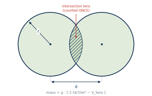
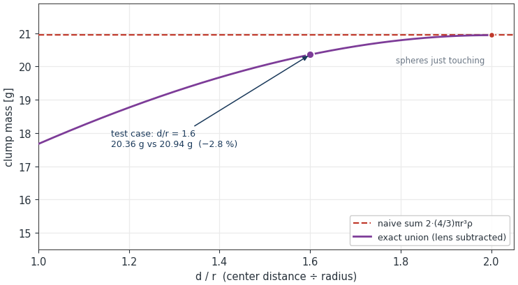
A clump is a rigid body made of overlapping spheres (Chapter 3.14). The verification covers the whole chain: the mass properties obtained from the geometric union of the spheres, the load distribution among the pebbles in contact, the response to constant force and torque, the invariants of central and eccentric impact, JKR cohesion on the clump, and the convergence order of the orientation integration.
Result
0 failures across 17 checks.
| Quantity | Expected | brixDEM |
|---|---|---|
| Mass scaling M ~ ρ·s³ | 0 | 0 |
| Inertia scaling I ~ ρ·s⁵ | 0 | 0 |
| Hertz equilibrium: overlap | 2.699789×10⁻⁵ | 2.699789×10⁻⁵ |
| Hertz equilibrium: total load | 0.205538 | 0.205538 |
| Load distribution among pebbles | 0 | 0 |
| Constant force: Δv = F·t/M | 0.5499863 | 0.5499862 |
| Constant torque: ΔL = τ·t | 5.382208×10⁻⁶ | 5.386167×10⁻⁶ |
| Central impact: restitution | 0.7 | 0.7203921 |
| Central impact: P / L conservation | 0 / 0 | 0 / 1.34×10⁻¹⁹ |
| Eccentric impact: restitution | 0.7 | 0.7202585 |
| Eccentric impact: P / L conservation | 0 / 0 | 0 / 2.05×10⁻¹⁴ |
| JKR on clump: pull-off force | 5.654867×10⁻³ N | 5.654954×10⁻³ N |
| JKR on clump: rupture distance | 1.640308×10⁻⁶ m | 1.640452×10⁻⁶ m |
| Rigidity: distance between pebbles | 0 | 1.39×10⁻¹⁷ |
| Orientation: \|q\| − 1 | 0 | 0 |
| Temporal order of orientation integration | 2 | 2.001639 |
11. Liquid bridge: separation, rupture and viscosity
What this case verifies
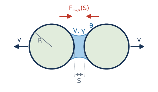
Two spheres form a bridge on touching and then separate. Force at each separation is compared with the Mikami correlation, together with the distance at which the bridge ceases to act. A second test adds normal and tangential motion to check Nase’s viscous resistance. Equations and conventions are in 3.15.
Parameters and procedure
| Panel / condition | Value |
|---|---|
| Spheres | R = 1 mm; ρ = 1×10⁶ kg/m³; E = 1×10⁷ Pa; ν = 0.30; e = 1; μ = 0 |
| Prescribed bridge | γ = 0.072 N/m; θ = 0°; V̂ = 0.002; V = 2×10⁻¹² m³; CGF = 1 |
| Initial condition | Overlap 2×10⁻⁷ m; axial velocities −0.01 and +0.01 m/s; zero gravity. |
| Timestep | Δt = 1×10⁻⁷ s |
| Viscous test | η = 1000 mPa·s; S₀ = 1×10⁻⁶ m; v₂,t = 0.01 m/s |
| Sphere–plane variant | R = 1 mm; θ = 20°; V̂ = 0.002 |
In the GUI, use two spheres, zero gravity and prescribed bridge volume with zero liquid contents (10.9); record force and surface separation until rupture. In the second test, enable viscosity and tangential velocity. The high density is artificial: it limits acceleration while reading the curve and is not an ore property. Pointwise comparison requires controlled position and force recording; the quick plotter does not directly provide a surface-separation axis.
Result
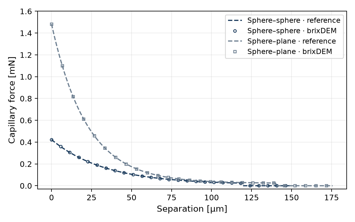
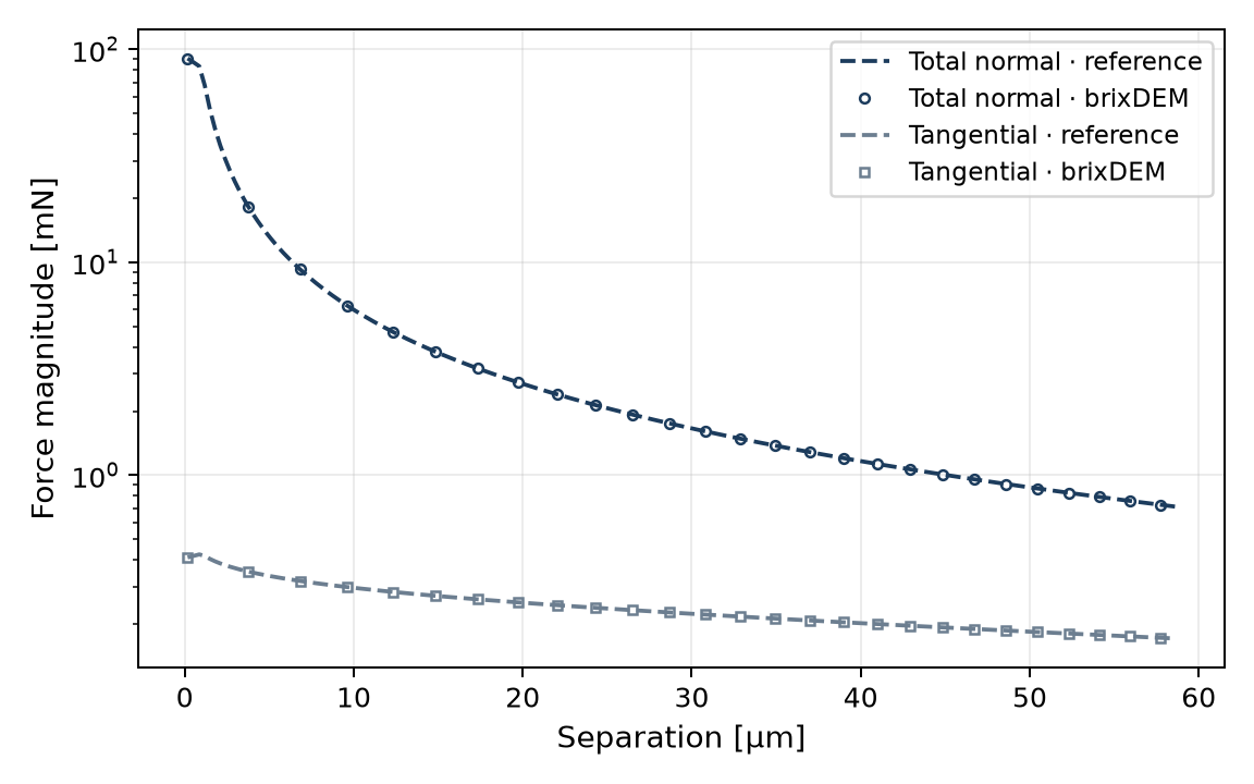
| Quantity | Reference | brixDEM / error | Criterion |
|---|---|---|---|
| F(h) | Mikami, Eqs. (3.56)–(3.58) | 4.42×10⁻¹⁶ maximum relative error | ≤ 1×10⁻⁶ |
| Rupture: equal spheres | 119.670 µm | 119.669 µm; 0.00084% | ≤ 0.01% |
| Normal viscous force | Nase, Eq. (3.60) | 5.61×10⁻⁵ maximum relative error | ≤ 1×10⁻⁴ |
| Tangential viscous force | Nase, Eq. (3.60) | 6.65×10⁻⁶ maximum relative error | ≤ 1×10⁻⁴ |
Additional check: liquid conservation
In migration mode, repeat bridge formation and rupture with dry-basis contents of 5% and 1%, liquid density 1000 kg/m³ and relative bridge-volume limit 0.05. Liquid should move from film to bridge and return without changing the inventory of a closed system.
| Quantity | Reference / result |
|---|---|
| Initial films | 2.094395×10⁻⁷ m³; 4.188790×10⁻⁸ m³ |
| Formed bridge volume | 5×10⁻¹¹ m³ |
| Maximum relative inventory drift | 2.11×10⁻¹⁶; criterion ≤ 1×10⁻¹² |
For compatibility with clumps and breakage, see 28.7.
Code accuracy × model accuracy
The errors in the table above compare the solver with the same Mikami equation: they prove the law is implemented correctly, not that it reproduces a real bridge. The uncertainty of the model itself is much larger and can be estimated by comparing Mikami with other published solutions for the same case (equal spheres, R = 1 mm, V̂ = 0.002, θ = 0°):
| Quantity | Mikami (used in BrixDEM) | Independent reference | Difference |
|---|---|---|---|
| Force at contact, F/(2πRγ) | 0.935 | Derjaguin limit: 1 (V → 0) | −6.5% |
| Rupture distance | 119.67 µm | Lian et al. (1993): (1+θ/2)·V1/3 = 125.99 µm | −5.0% |
| Rupture distance | 119.67 µm | Willett et al. (2000): (1+θ/2)(V̂1/3+V̂2/3/10)·R = 127.58 µm | −6.2% |
| Rupture at V̂ = 0.001 / 0.01 / 0.05 | — | Willett et al. (2000) | −6.4% / −6.0% / −6.4% |
12. Liquid bridge with coarse-graining
What this case verifies
The same local interaction is compared at CGF 1, 2 and 4. The reference is the scaling of Eq. (3.64): forces four and sixteen times larger, respectively, at equal relative surface velocities. This supplements case 11; it does not compare equipment throughput or mixing.
Parameters and procedure
| Field | Physical value at CGF = 1 |
|---|---|
| Particles | R₁ = R₂ = 1 mm; ρ = 2500 kg/m³; E = 1×10⁵ Pa; e = 1; μ = 0 |
| Liquid | γ = 0.072 N/m; η = 1 mPa·s; θ = 17.1887°; V̂ = 0.002; S₀ = 1 µm |
| Measurement state | h/rₚ = 0.02; v = 0.02 m/s; ω = 0; Δt = 1×10⁻¹² s |
Form a bridge, set a controlled separation and measure the capillary and each viscous contribution separately. Repeat with enlarged geometry at CGF 2 and 4 while retaining physical input properties: conversion is applied once (10.7). The numerical test repositions the bridge after formation to isolate the law; it is not a free trajectory reproduced through animation alone.
Result
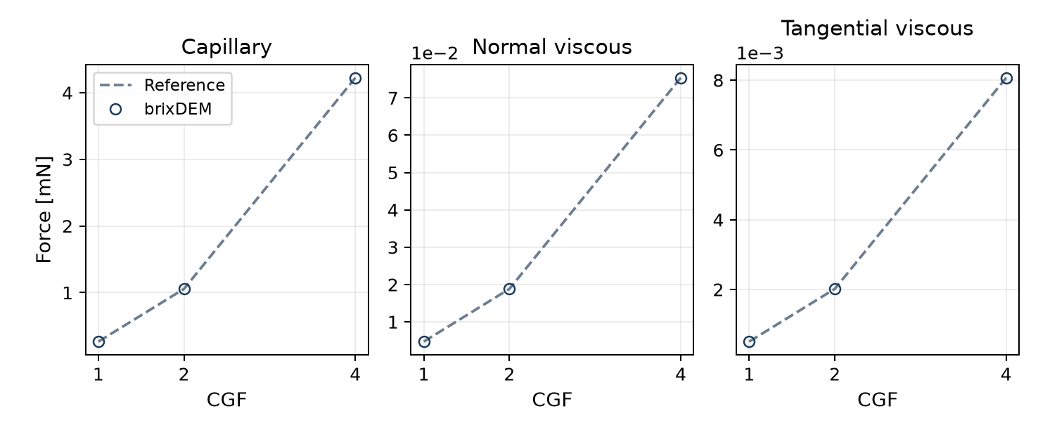
| CGF | Capillary [mN] | Normal viscous [mN] | Tangential viscous [mN] |
|---|---|---|---|
| 1 | 0.264005 | 0.00471239 | 0.000504326 |
| 2 | 1.05602 | 0.0188496 | 0.00201730 |
| 4 | 4.22408 | 0.0753982 | 0.00806922 |
13. Ab-T10/PRM breakage: DWT impact and progeny
What this case verifies
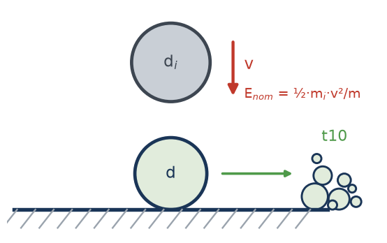
A breakable sphere rests on an anvil and is struck by a steel sphere. Work assigned to the event determines t10 and the fragment distribution; the product masses must sum to the parent mass. This virtual DWT connects impact mechanics to PRM replacement, while supplementary checks isolate selection, size and damage. Formulation is in 3.16.
Parameters and procedure
| Panel / condition | Value |
|---|---|
| Breakable body | d = 5.5 mm; ρ = 2930 kg/m³; E = 52 GPa; ν = 0.25 |
| Steel impactor and anvil | dᵢ = 12 mm; ρᵢ = 7800 kg/m³; Eᵢ = Ewall = 182 GPa; νᵢ = νwall = 0.30 |
| Ab-T10/PRM | S = 0.002 kg/J; dref = 5 mm; Emin,ref = 100 J/kg; A = 67.7%; seed = 0 |
| Contact / integration | Hertz–Mindlin; e = 1; μ = 0; g = 0; Δt = 5×10⁻⁸ s |
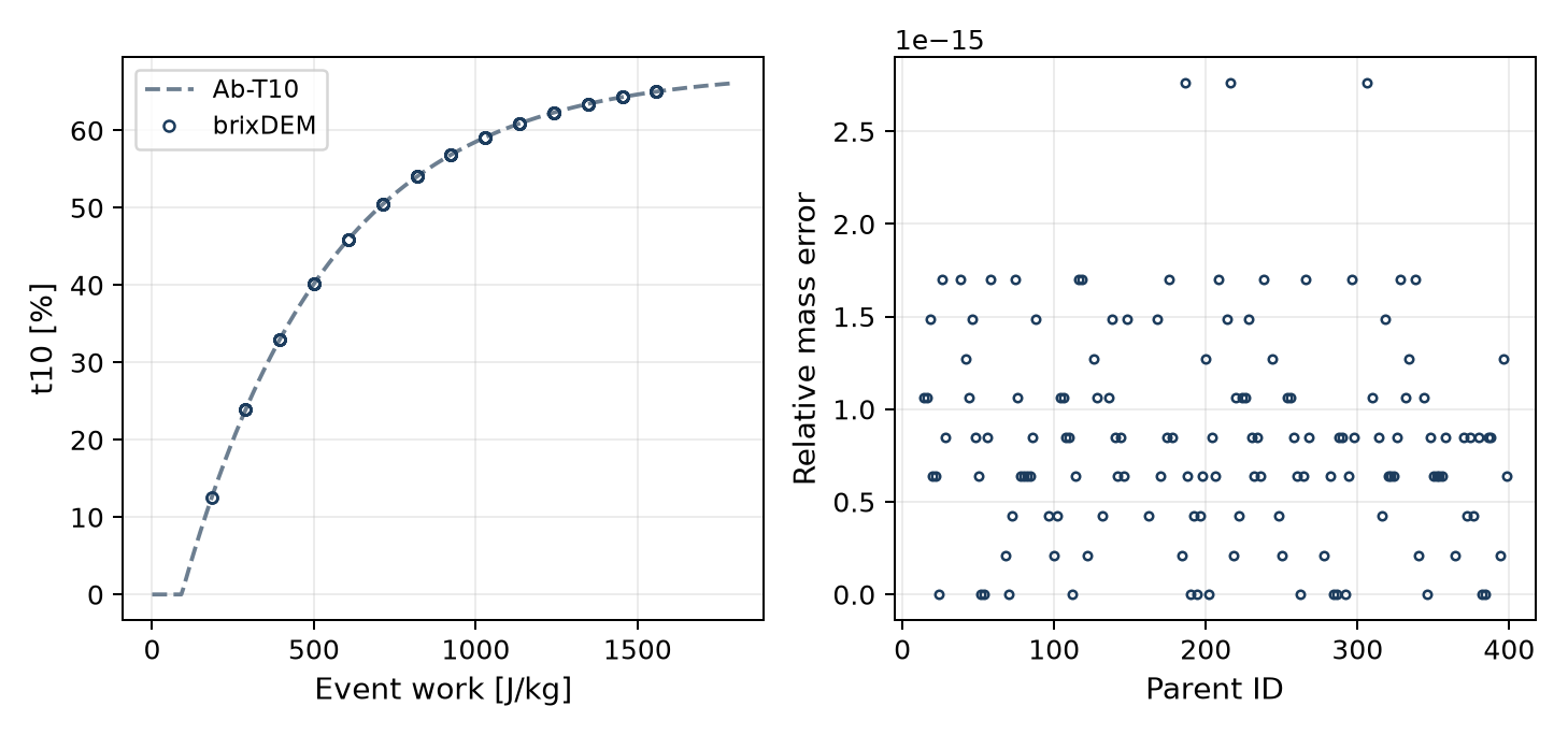
| Energy sweep | 200 independent pairs; initial impactor kinetic energy of 100–2000 J/kg of body mass; 4000 steps. |
Set the breakable material to Damage + replacement (10.10), keep the impactor unbreakable and set its velocity for the target energy. Comparison uses work actually assigned to the body, not nominal impactor energy. The campaign contains 139 fractured parents. Statistical reproduction across energies requires independent impacts and event recording; a single animation does not reproduce the full population.
Result: t10 and mass
| Quantity | Reference / criterion | Result |
|---|---|---|
| t10 | Eq. (3.69), using event work | Maximum difference ≤ 1.5×10⁻¹⁴ pp |
| Child and fines masses | Recover parent mass; relative error ≤ 1×10⁻⁹ | 2.76×10⁻¹⁵ maximum error |
Fragment-distribution check
To separate PRM sampling from impact mechanics, fix t10 = 20% and generate 10,000 families for each progeny law. Compare mean mass passing with the prescribed distribution, rather than sphere count.
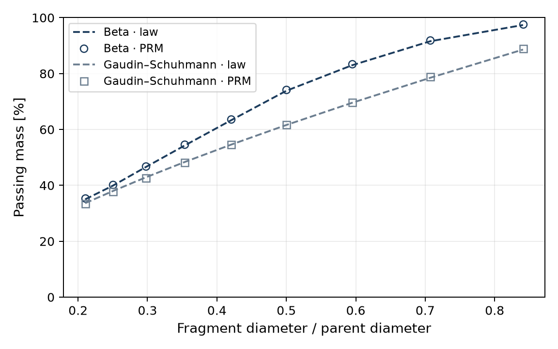
The maximum absolute difference in fractional passing is 0.0046 for Beta and 0.0047 for Gaudin–Schuhmann: approximately 0.46 and 0.47 percentage points. Fragment discretisation and sampling explain the difference between a continuous curve and a finite population.
Supplementary checks: selection, size and damage
For selection, use 1,000 fresh bodies per energy with the tabulated properties and replacement disabled. For size effects, repeat at diameters of 2.5, 5.5 and 11 mm. For repeated impacts, retain damage across five impacts with mean specific work of 194.96 J/kg.
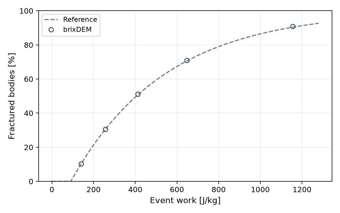
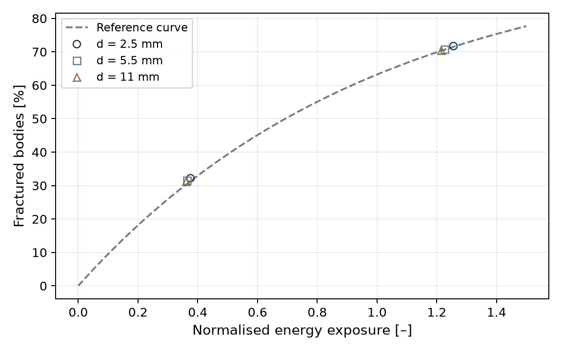
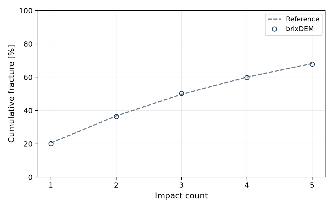
| Event E [J/kg] | Reference P [%] | Fractured [%] | Difference [pp] |
|---|---|---|---|
| 140.63 | 10.36 | 10.20 | −0.16 |
| 256.59 | 30.55 | 30.60 | +0.05 |
| 411.92 | 50.65 | 51.20 | +0.55 |
| 647.96 | 70.64 | 70.90 | +0.26 |
| 1156.05 | 90.40 | 90.90 | +0.50 |
Progeny law × published family
The Beta law (default) uses the incomplete beta function with the parameters of Tavares & das Chagas (2021, Table 3), fitted to 40 materials (rocks, ores and clinker, excluding iron ore): tn = 100·I(t10/100; αn, βn). The Gaudin–Schuhmann option uses a single exponent obtained from t10, tn = (1/n)α with α = ln(t10)/ln(0.1). Percent passing at 1/2, 1/4, 1/25 and 1/75 of the parent size:
| t10 | Beta (published family) — t2 / t4 / t25 / t75 | Gaudin–Schuhmann — t2 / t4 / t25 / t75 |
|---|---|---|
| 10 % | 47.5 / 20.3 / 5.7 / 3.2 | 50.0 / 25.0 / 4.0 / 1.3 |
| 20 % | 73.8 / 39.9 / 11.5 / 6.4 | 61.6 / 38.0 / 10.5 / 4.9 |
| 30 % | 88.0 / 56.8 / 17.6 / 9.8 | 69.6 / 48.4 / 18.6 / 10.5 |
For t10 ≥ 20%, Gaudin–Schuhmann underestimates the coarse part by up to 12–19 percentage points (t2). Prefer Beta unless material data justify the other law. Iron ores fall outside the published family (lower t2 and higher t75 for the same t10); for them, the default parameters are not an adequate estimate. Fines below the smallest fragment are represented by dummy particles; the power-law extension suggested in the same reference is not applied.
Energy assigned to the body and stiffness
Ab-T10 uses the work absorbed by the body, split between both sides of the contact by η = kpartner/(kbody+kpartner), not the nominal impactor energy. The parameters are therefore valid only at the stiffness at which they were calibrated. Example with fixed S and Emin, sphere against a 200 GPa wall, 72 J/kg per impact and 10 impacts:
| Body Young's modulus | η (body share) | Fraction fractured |
|---|---|---|
| 5.2 GPa | 0.975 | 76.2% |
| 52 GPa | 0.798 | 66.0% |
| 208 GPa | 0.498 | 44.5% |
Uniform reduction of Young's modulus. When Young's modulus of all materials — particles, impactor and walls — is multiplied by the same factor, η does not change and the response is preserved. Same test (10 impacts of 72 J/kg, 128 bodies per shape, calibration not refitted; particle/wall 52/200 GPa as reference):
| Shape | Factor 1 (52/200 GPa) | Factor 0.1 | Factor 0.01 |
|---|---|---|---|
| Sphere | 60.16% | 60.16% (+0.00 p.p.) | 60.16% (+0.00 p.p.) |
| Pair clump | 62.50% | 62.50% (+0.00 p.p.) | 63.28% (+0.78 p.p.) |
| Tetra clump | 59.38% | 60.16% (+0.78 p.p.) | 61.72% (+2.34 p.p.) |
η = 0.798 for all three factors. For spheres, the fraction with a first fracture is identical up to a 100× reduction; for clumps, the difference stays within 1–3 bodies out of 128. Uniform reduction is therefore the consistent way to gain timestep without recalibrating Ab-T10 for this type of impact. The test covers repeated isolated impacts; it does not cover confined beds or the fragment distribution.
14. Evidence summary and limits
| # | Case | Verified quantity | Result |
|---|---|---|---|
| 1 | Normal restitution | e = |v_out/v_in| | 10.1% at e=.5; ≤2.6% at e≥.7; large deviations at low e |
| 2 | Oblique collision | coupling Δω/Δv_t | OK 5.5 % (torque) |
| 3 | Sliding into rolling | v_f, ω_f, t_s | OK 0.05 % |
| 4 | Ramp rolling | a = 5/7·g·sinθ | OK < 0.1 % |
| 5 | Ramp sliding | a = g(sinθ−μcosθ) | OK < 0.01 % |
| 6 | Rolling threshold | θc = arctan(μ_r) | OK (16 to 17°) |
| 7 | Braking by rolling | a = 5/7·μ_r·g | OK 0.1 % |
| 8 | JKR adhesion (particle) | F = 3π·γ·R_eff and rupture gap | OK < 0.1 % |
| 8b | JKR adhesion (wall) | pull-off, rupture gap and F(δ) curve | OK < 0.1 % |
| 9 | Free-body 6-DOF | torque-free rotation; eccentric impact and reactions | Measured coupling: 25/25; Part A free rotation: reference without solver result |
| 10 | Clumps | mass/inertia, invariants, JKR and orientation | OK; 0 failures across 17 checks |
| 11 | Liquid bridge | Force, rupture, viscosity and inventory | Rupture: 0.00084%; viscosity: relative error ≤ 5.61×10⁻⁵ (code × equation). Model × published correlations: 5–7%; no experimental validation |
| 12 | Bridge + coarse-graining | Local force scaling | Maximum relative error 6.98×10⁻⁹; no macroscopic validation |
| 13 | Ab-T10/PRM | DWT, progeny, selection, size and damage | Mass: relative error 2.76×10⁻¹⁵; progeny ≤ 0.5 p.p. from the prescribed curve; uniform Young reduction preserves selection. PSD of a specific material not validated |
These cases check laws and balances under the stated conditions. When reproducing a test, compare the same quantity, population and measurement interval. Agreement with an equation does not replace experimental validation of a material or equipment; calibration and physical-comparison procedures are in Chapter 18.