
CHAPTER 24
Tutorial 4 — Clumps + hinged 6-DOF body
Step-by-step reproduction of the video case: a belt surface carries clumps to a hinged gate that opens under granular load.
What you will build. Two independent STLs:
conveyor_belt_static.stl, which remains in place but receives Belt surface motion, and hinged_flop_gate_6dof.stl, which receives free 6-DOF dynamics and a hinge. Then you configure the domain, materials, clump, contacts, inlet, solver, and results.Follow this order. Geometry (Belt first, 6-DOF second) → Domain → Materials and interactions → Insertion → Setup → Run → Results. Save after each module.
24.1 Geometry: configure Belt first and the 6-DOF body second
Step 1 — import and identify both STLs
- Create a new project, save it as
Tutorial4_Clumps_6DOF.brixdemproject, and open Geometry › STL. - Click Import STL and choose
conveyor_belt_static.stl. Then importhinged_flop_gate_6dof.stl. - Confirm that they appear as separate items. They cannot be merged: the belt receives prescribed motion while the gate responds freely to forces.
- Check scale, position, and orientation. In the video, the belt is on the right and delivers material to the gate on the left. If the CAD geometry was exported in millimetres, apply scale 0.001.
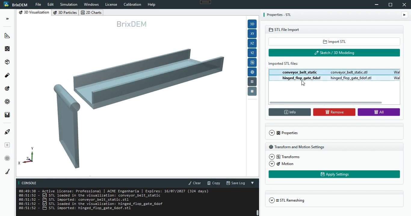
Step 2 — apply Belt to conveyor_belt_static.stl
- In the STL list, click
conveyor_belt_static. Check the selected name before continuing. - Open Transformations and motion settings › Motion.
- Under Motion Type, choose Belt/Conveyor. Under Belt mode, choose Linear.
- Enter linear velocity X = 1.5; Y = 0; Z = 0 m/s, as shown in the video.
- Keep Use local geometry direction enabled. If particles travel away from the gate, change X to −1.5.
- Click Apply Settings. The STL does not translate: Belt moves only the contact surface, like a real conveyor belt.
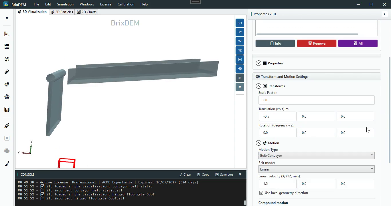
conveyor_belt_static first, then apply linear Belt/Conveyor with vector (1.5, 0, 0) m/s. Original Portuguese-interface capture.Common mistake. Do not apply Linear body motion and do not apply Belt to the gate. The selected item must be
conveyor_belt_static.Step 3 — configure hinged_flop_gate_6dof.stl as a free body
- Now select
hinged_flop_gate_6dof. - Under Motion Type, choose Free-body 6-DOF.
- Choose Free — 6 degrees of freedom and click Apply preset. The hinge is added next.
- Assign the Wall material with density 7800 kg/m³ and click Compute STL mass, centre and inertia + material density.
- For the video mesh, the GUI computes volume ≈ 0.038695 m³, mass ≈ 301.823 kg, and centre of mass near (0.2200, 1.1310, 0) m. Always calculate; do not type these values for another mesh.
- Leave initial orientation, linear velocity, and angular velocity at zero.
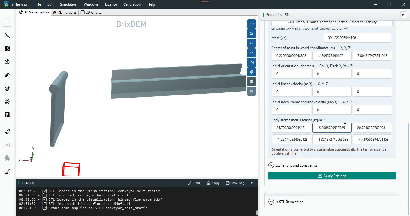
Step 4 — constrain the gate with a hinge
- Expand Excitations and constraints. Keep external force and torque at zero and leave manual locks cleared.
- Enable Physical hinge — keeps the body fixed at one pivot and free about one axis.
- Enter global pivot (0.22, 0, 0) m and global axis (0, 0, 1).
- The pivot must match the cylindrical joint centre. The Z axis permits swinging in the flow plane.
- Leave hybrid drive, springs/dampers, and limits disabled, then click Apply Settings.
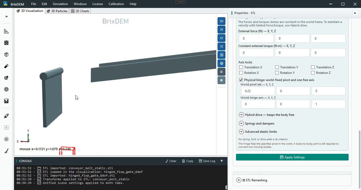
24.2 Domain: include feeding, transport, and opening
- Open Domain and click Fit to Geometry.
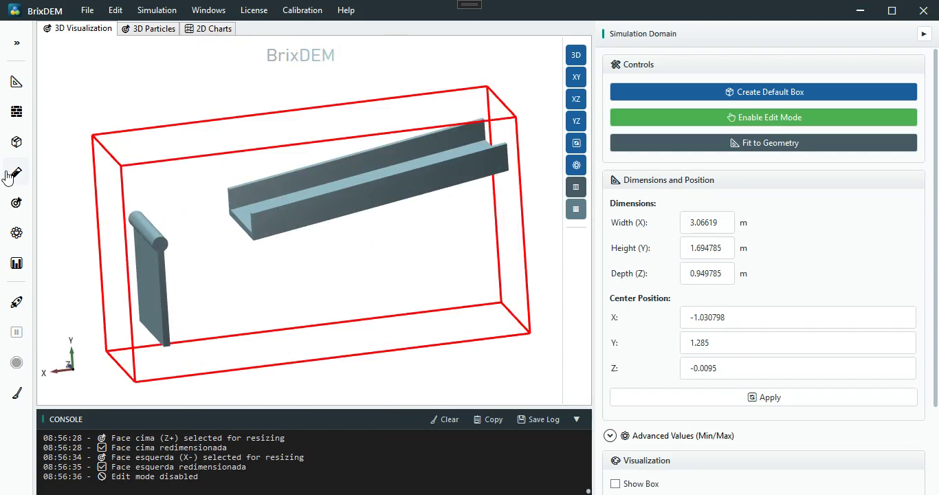
- Enable edit mode and drag the red box faces to include the inlet disk, complete belt, closed gate, full opening arc, and discharge fall region.
- In the video, the final values are approximately X width 3.06619 m, Y height 1.694785 m, Z depth 0.949785 m, and centre (−1.030798, 1.285, −0.0095) m.
- Click Apply and disable edit mode. These values reproduce this geometry; adjust visually for any changed position.
24.3 Materials, clump shape, and interactions
Step 1 — create both materials
- Open Materials, click Add, and create Wall with density 7800 kg/m³. Assign it to both STLs.
- Add particle material clump with density 2500 kg/m³ and base radius 0.005 m. Save before opening the clump editor.
- Young’s modulus and Poisson’s ratio must come from the real material or calibration. Density defines mass; restitution and friction belong to contact pairs.
Step 2 — turn the material into a multisphere clump
- Select clump and click Define Clump….
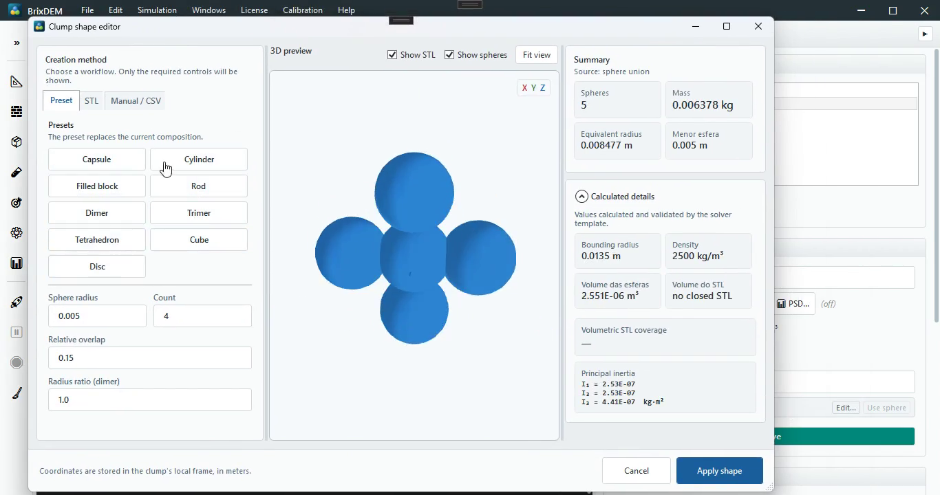
- Choose the video multisphere preset and enter radius 0.005 m, count 4, and relative overlap 0.15.
- Check the preview, mass, equivalent radius, and tensor. Click Apply Shape; closing without applying keeps the previous spherical shape.
Step 3 — create both contact pairs
- Open Configure Material Interaction.
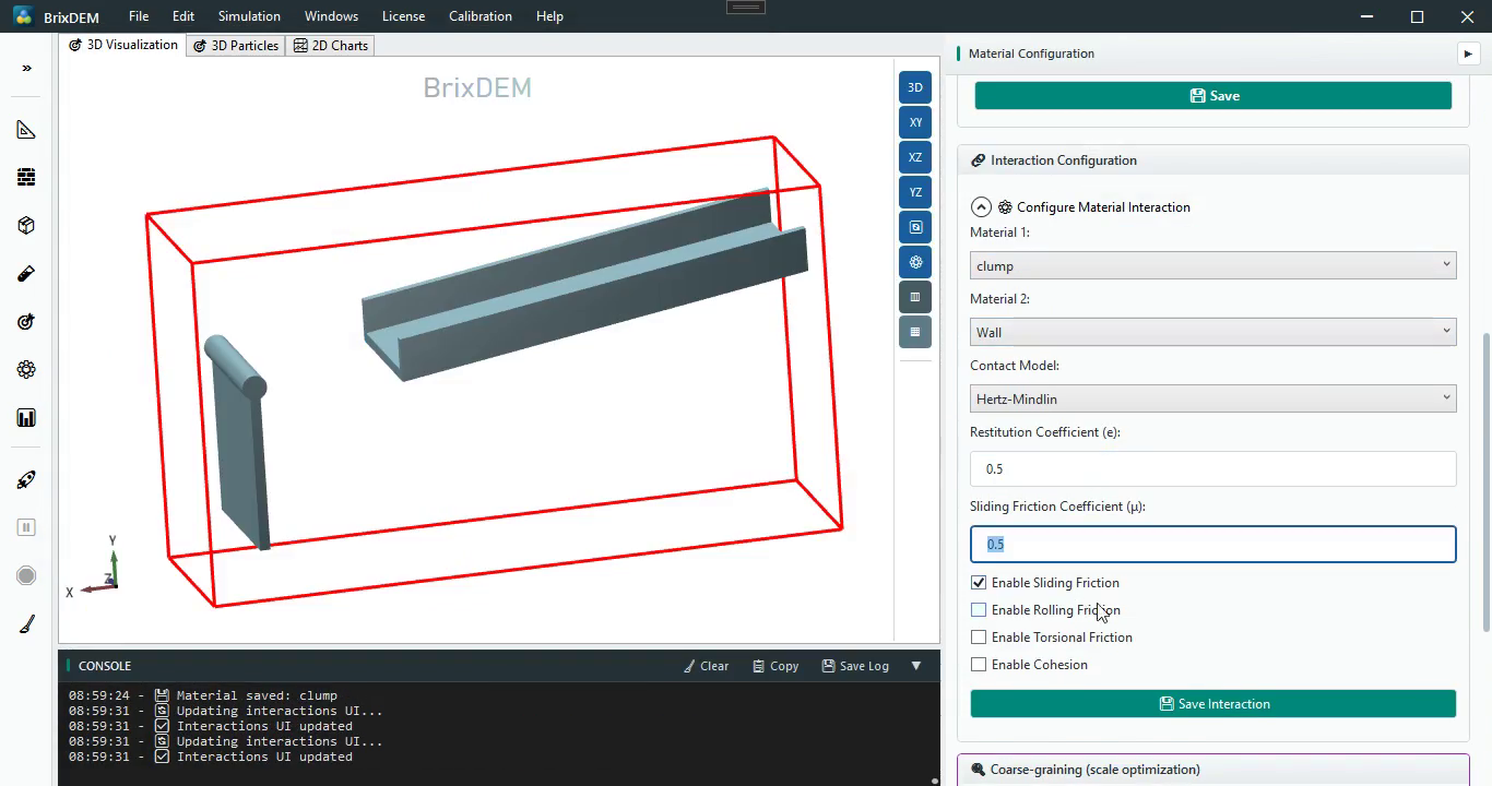
- Choose Material 1 = clump and Material 2 = Wall. Use Hertz–Mindlin, restitution 0.5, enable sliding friction, enter 0.5, and click Save Interaction.
- Change Material 2 to clump, keep the same values, and save clump ↔ clump.
- Confirm both pairs. The first enables belt transport and gate loading; the second controls packing and flow between clumps.
24.4 Insertion: feed clumps at the belt entrance
- Open Insertion, choose Inlet, and select a circular shape.
- Select clump and place the disk above the belt entrance without intersecting walls.
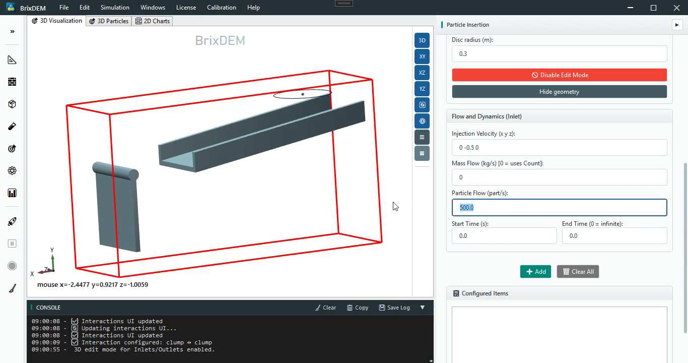
- Set disk radius to 0.3 m.
- Set injection velocity to (0, −0.5, 0) m/s, pointing toward the belt.
- Leave mass flow at 0 to use count and enter 500 particles/s.
- Use start 0 s and end 0, meaning active until the run ends.
- Click Add. Verify
inlet_CLUMPunder Configured Items; filling fields alone does not create it.
24.5 Setup: configure the solver
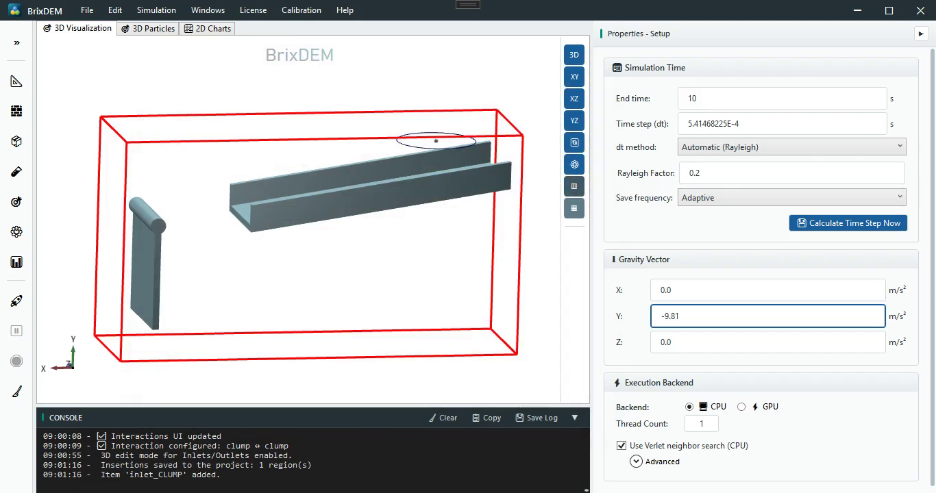
- Open Setup and set end time to 10 s.
- Choose Automatic (Rayleigh), factor 0.2, and click Calculate Time Step Now. The video obtains approximately 5.41468225×10⁻⁴ s.
- Choose Adaptive save frequency.
- Set gravity to (0, −9.81, 0) m/s².
- Select CPU or GPU. The video uses CPU; set the thread count available on the computer.
- Save the project and choose an empty results folder.
24.6 Run and verify physical behaviour
- Start a new Run. First confirm that clumps spawn above the belt without an explosive overlap.
- Check that Belt carries them to the gate. If they move backwards, stop, reverse the Belt vector, apply it, and start another Run.
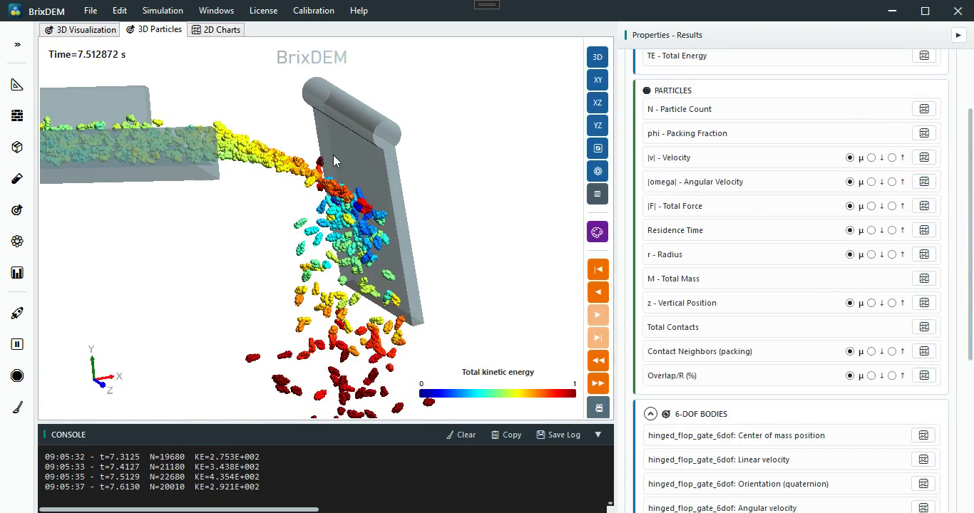
- Clumps must accumulate against the gate; contact force and torque rotate it about the pivot and release the material.
- The body may oscillate, but the pivot must not translate. Translation indicates a missing hinge or the wrong body configured.
- Under 3D Particles, use velocity magnitude or kinetic energy to visualize acceleration after opening.
24.7 Results: particles and gate motion
Particle results
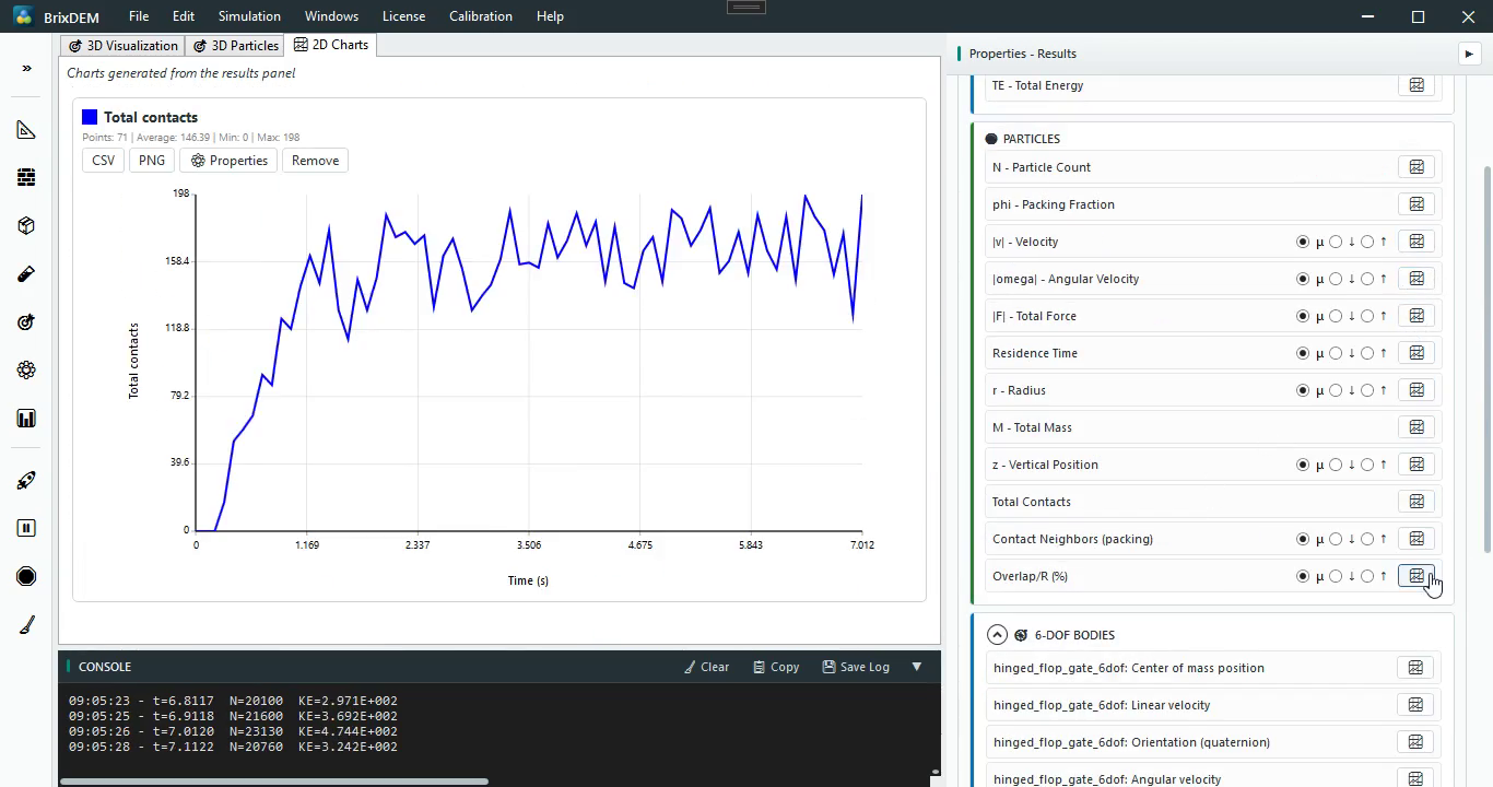
- Open Results › Particles. Available groups include count, packing fraction, velocity, angular velocity, total force, residence time, radius, total mass, vertical position, and contacts.
- Plot Total contacts: the initial rise represents bed formation; later oscillations follow loading and discharge through the gate.
- Plot mean velocity as well to identify jet acceleration and regime stabilization.
6-DOF body results
- Expand 6-DOF Bodies and locate
hinged_flop_gate_6dof. - The seven series are centre-of-mass position, linear velocity, quaternion orientation, angular velocity, resultant force, resultant torque, and mechanical power.
- For this hinge, monitor mainly angular velocity Z, torque Z, and quaternion. Force and torque show granular loading; oscillations describe opening and return.
- Use centre-of-mass position to verify the constraint: it must follow the pivot arc without free drift.
Final checklist. Belt only on the conveyor; Free 6-DOF and hinge only on the gate; domain contains the full arc; materials and two contact pairs saved; clump applied; inlet added; timestep recalculated; particle and 6-DOF results available.