
3D Particles and Snapshots
GPU accelerated viewing of particle snapshots, with coloring and playback controls.
15.1 3D Particles Tab
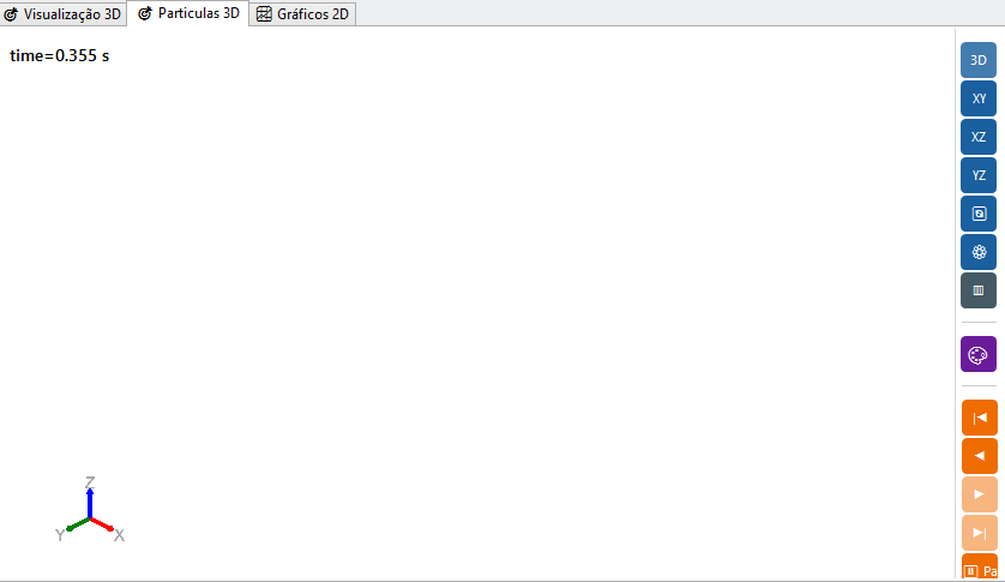
The 3D Particles tab uses a dedicated, GPU-accelerated 3D rendering engine for the efficient visualization of hundreds of thousands of particles — separate from the engine used by the pre-processing 3D Visualization tab (Chapter 14). It shows: particles colored by the selected scalar; colorbar/legend with minimum and maximum values; current snapshot time; and playback controls (previous, next, play, stop, reverse).
15.2 What is a snapshot and how it is recorded
One snapshot (or frame) is a complete photograph of the state of all particles in an instant: position, velocity, angular velocity, force, torque, radius, mass and material of each. The snapshot sequence forms the "film" of the simulation you play in the 3D Particles tab and use in plots.
Snapshots are recorded by the solver during execution, controlled by the field Save frequency (Save Count) of the Setup panel (Chapter 12.5). Solver does not record every step - it would generate thousands of files - but every N steps. Each recording produces a file particles_NNNNNN.bin (binary format) DEM2), where the number is the simulation step:
| RECORDING METHOD | BEHAVIOR | WHEN TO USE |
|---|---|---|
| Adaptive | DEM2 snapshots at the same cadence as the visual stream (~300 per simulation): scalars and residence in every frame, no disk cap | Default; suitable for most cases |
| Fixed interval (every N steps) | Record every N solver steps | When you need uniform and controlled temporal spacing |
.bin, the solver also records energy.csv, contact_stats.csv and other CSVs (Appendix A) - these do not depend on the Save Count of particles.How to view snapshots
No need to manually open the files. With the project open (or during execution), the tab 3D particles locates .bin in the results folder and loads the entire sequence automatically. From there:
- Click Last snapshot and 3D to frame the scene;
- Choose color scalar (speed, force, height...) on the palette button - see 15.3 and 15.4;
- Use the Playback controls (first/previous/play/next/last) to move through time - see 15.5;
- To compare moments on the same scale, fix the minimum/maximum range of colorbar.
15.3 Automatic loading
When a simulation is open or running, the software automatically searches for snapshots .bin in the results folder and loads the set. New snapshots appear dynamically during execution. Snapshots follow binary format DEM2 (see Appendix A).
15.4 Color variable (scalar coloring)
Each particle is colored by one scalar mapped into a color palette. Changing the scalar reveals different aspects of the same instant - speed, force, height, contacts - without reprocessing the simulation. The scalar is chosen in the colorbar configuration (next section) from the available variables:
| SCALAR | WHAT IT REVEALS |
|---|---|
| Speed | Fast and slow zones; jets, avalanches, dead regions |
| Components vx, v y, v z | Predominant flow direction along each axis |
| Angular velocity | Intense rolling (agitation, drum bed) |
| Force | Force chains, loading and impact locations |
| Position z | Stratification by height; useful for segregation and filling |
| Radius r | Granulometric distribution / segregation by size |
| Material / category (info) | Visually identifies each species/particle material |
Real examples of scalar coloring in the GUI appear in the tutorials: Figures 21.4 and 21.5 (mixer) and 22.5 (drum with flights) show particles colored by |v| and by kinetic energy in the 3D Particles tab itself.
15.5 Colorbar Settings
The scaling configuration button allows you to adjust the displayed variable, the color palette, the minimum/maximum interval (automatic or manual), the colorbar position (one of the four screen corners) and the caption font/size. Setting the interval manually is essential to compare snapshots or different cases on the same scale.
15.6 Snapshot navigation
| CONTROL | FUNCTION |
|---|---|
| First / Last | Jump to start or end |
| Prev / Next | Forward/return a snapshot |
| Reverse Play / Play Forward | Play Backwards / From Current Snapshot |
| Stop | Pause playback |
Use slow playback for the diagnosis of spot events (impacts, pile formation) and fast playback for an overview of the steady regime.
15.7 Video recording
In addition to going through the snapshots on the screen, it is possible to export an animation from the visualization as a video file. FPS, timescale and codec options should be configured in the viewing properties before starting the recording. Don't confuse this recording of video (visual output) with recording of snapshots .bin by the solver (data, section 15.2).
15.8 Available color palettes
The palette chosen in the colorbar settings (15.5) maps the scalar value to a color, from the minimum to the maximum of the range. BrixDEM offers 13 palettes:
| PALETTE | GRADIENT (min → max) | WHEN TO USE |
|---|---|---|
| Jet | General default, high contrast - but not perceptually uniform; avoid it for fine quantitative reading | |
| Viridis | Perceptually uniform and colorblind-friendly; a good default for reports | |
| Turbo | Corrected rainbow - more uniform than Jet, keeping high contrast | |
| Plasma | Uniform, high contrast - reads well on dark backgrounds too | |
| Inferno | Uniform, good for light backgrounds or print | |
| Magma | Uniform, softer tones - good for overlaying on geometry | |
| Cividis | Uniform and optimized for color-vision deficiency (deuteranopia/protanopia) | |
| Rainbow | Classic rainbow - strong visual contrast, but can suggest bands that aren't in the data | |
| Spectral | Diverging - ideal for signed quantities (e.g., vx, vy, vz components around zero) | |
| Blue-Red | Simple 2-color diverging scale - opposite extremes, no neutral center tone | |
| Coolwarm | Diverging with a neutral center - good for deviation around a reference value | |
| Thermal | Thermal-camera style - intuitive for force/power/"hot" quantities | |
| Gray | Grayscale - for black-and-white print or for overlaying contours |
15.9 Geometry and particle synchronization
Play and snapshot use the same solver-state instant: geometry and particles should correspond to the same frame. If a result file did not record the required field/frame, the viewer cannot reconstruct it later.