
Tutorial 2 — Rotary drum with flights (ball mill)
Case recorded on video: drum with flights created in the Sketch Modeler, instant fill at the axis, ramped rotation and reading of overlap, energy and power.
This tutorial reproduces the Drum T2 case from the tutorial video: a drum with flights (typical ball-mill configuration) created in the Advanced tab, filled by a cylindrical inlet at the axis and set to spin with a ramp. The post-processing focus is numerical diagnosis — overlap, kinetic energy, force and power on the body.
22.1 Case overview
| ITEM | VALUE USED |
|---|---|
| Geometry | Drum with flights (Sketch › Advanced › Rotary drums › Flights), 8 flights, axis at the origin |
| Motion | Rotational, ω = (9; 0; 0) rad/s, velocity ramp starting at 1 s |
| Materials | New particle material (small radius, ρ 1000 kg/m³, reduced E); wall with the same properties |
| Interactions | Particle↔particle and particle↔wall: eₙ 0.5, μ 0.5, rolling enabled (uncalibrated values) |
| Inlet | Cylinder at the axis: base (−0.025; 0; 0), top (0.025; 0; 0), radius 0.08 m; 5000 particles, instant fill |
| Setup | End time 10 s, automatic Δt (Rayleigh), CPU 4 threads |
| Result | ≈ 1400 particles injected (overlap prevention); cascade with flights and chart-based diagnosis |
22.2 Step by step
Step 1 — Create the drum with flights
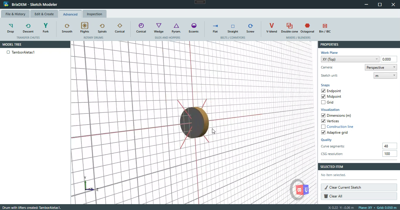
In Geometry › STL › Sketch / 3D Modeling, open the Advanced tab and, under Rotary drums, click Flights ("Drum with flights"). The parametric form defines the complete drum:
| FIELD | WHAT IT CONTROLS |
|---|---|
| Length | Drum depth along the axis |
| Outer diameter | Diameter of the cylindrical shell |
| Wall thickness | Shell thickness (affects only the geometry, not the wall physics) |
| Flight height | How far each flight reaches inwards — controls how much material is lifted per revolution |
| Flight thickness | Thickness of each inner blade |
| Flight count | How many equally spaced blades (8 in the video) |
Click Create. An important detail of the parametric geometry, highlighted in the video: the drum axis is created at the work-plane origin — in practice this means that in Step 2 the rotation center will simply be (0; 0; 0), with no need to measure the real mesh axis. Use Send (File & History tab) to push TamborAletas1 to the main window.
Step 2 — STL properties and motion
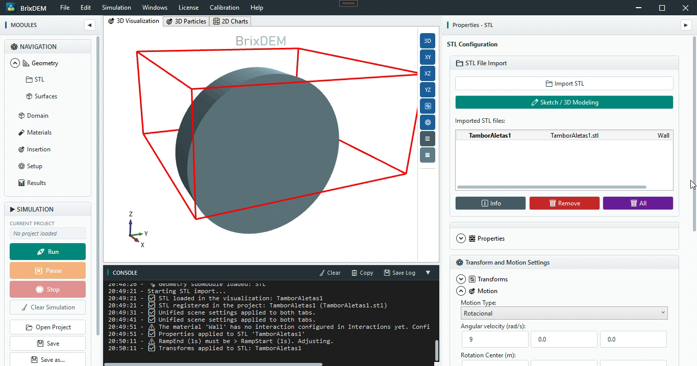
In the STL properties: confirm the wall material (Wall), reduce the body opacity (in the video, translucent white body) to see the interior, and enable force and torque measurement — it is what allows reading drum torque and power in post-processing. Under Motion:
- Type = Rotational, ω = (9; 0; 0) rad/s (≈ 86 rpm) — spin about X, the drum axis. The vector defines axis and magnitude at once;
- Rotation center = (0; 0; 0) — valid because the Sketch created the drum at the origin;
- Velocity ramp enabled starting at 1 s: the wall does not jump from rest to 9 rad/s in a single step, which would launch the particles in contact (Chapter 7.6).
Click Apply Settings and check in the console the confirmation of the transforms and the automatic ramp adjustment. Use the orthogonal views (XY/XZ/YZ) and the edge mode to verify the flight positions.
Step 3 — Domain and materials
Fit the Domain around the drum (Fit to Geometry). In Materials, create a new particle material with small radius, density 1000 kg/m³ and reduced elastic modulus — softer contacts lengthen the collision time and allow a larger Δt, standard practice in production (Chapters 19.8 and 25); edit the wall to the same elastic properties. In Interaction Configuration, establish all contact combinations:
| PAIR | VALUES IN THE VIDEO | ROLE IN THE CASE |
|---|---|---|
| Particle ↔ Particle | eₙ 0.5 · μ 0.5 · rolling on | Dissipation and interlocking of the cascading bed |
| Particle ↔ Wall | eₙ 0.5 · μ 0.5 · rolling on | Dragging of the material by the shell and the flights |
| Wall ↔ Wall | default | No physical effect here; defined to complete the pair matrix |
Step 4 — Inlet at the axis with instant fill
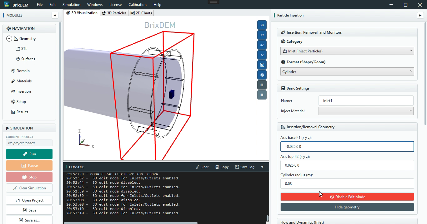
In Insertion, create an Inlet of Cylinder format aligned with the drum axis: base (−0.025; 0; 0), top (0.025; 0; 0) and radius 0.08 m. In the video the radius was reduced from the first attempt precisely so the cylinder does not touch the wall or the flights — particles born in contact with the geometry receive a huge force on the first step and destabilise the case. Injection direction along Y, 5000 particles, instant fill, and Add.
Step 5 — Setup, save and run
In Setup: end time 10 s, automatic Δt (Rayleigh) and CPU with 4 threads. Save the project in its own folder (in the video, BallMill_Tutorial02) and click Run. Not all 5000 particles enter: the solver prevents particles from being born overlapping each other or the geometry, and the case proceeds with ≈ 1400 particles. As said in the video, this is something to check consciously after instant injection: confirm in the console/count chart how many particles actually entered.
Step 6 — Chart-based diagnosis during the run
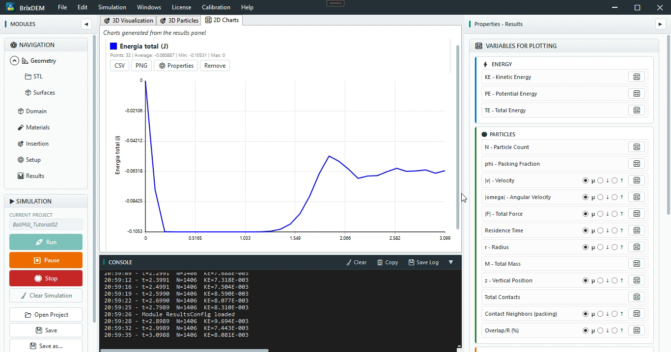
Open Results and plot the diagnostic variables while the case runs — each one answers a question:
| CHART | WHAT TO CHECK IN THIS CASE |
|---|---|
| Overlap/R (min/mean/max) | Peak right after the instant injection and drop to ~5 % — the bed relaxed; growing overlap would indicate insufficient Δt |
| KE — Kinetic energy | Rises when the ramp ends and the rotation reaches the regime; stabilises in the cascade |
| |v| — Mean velocity | Operating level; compare different rotation speeds |
| |F| — Total force | Mean load on the particles; peaks reveal strong flight impacts |
| Body force/torque | Load on the drum (requires the measurement enabled in Step 2) |
| P_mech — Power | Power to spin the material — an engineering quantity for the mill (Chapter 16.10) |
The panel also reports elapsed time, the estimated remaining time (ETA) and the time step in use — useful to decide whether to wait or interrupt and adjust.
Step 7 — Scalars in the visualisation
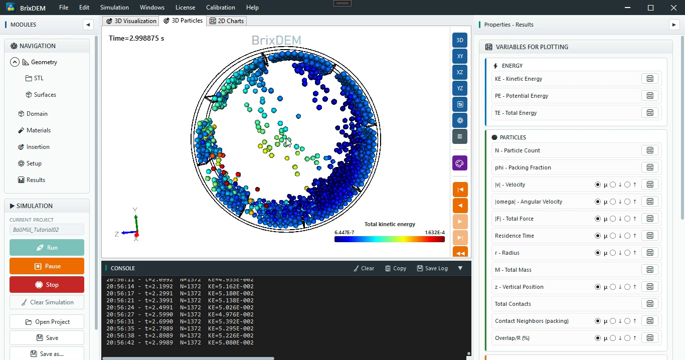
In the 3D Particles tab, use the scalar button to color the particles by total kinetic energy or by velocity. A trick used in the video: limit the colorbar range (e.g. 0 to 0.1) — with the automatic range, the few high values "steal" the scale and the whole bed turns blue; with the limited range, the contrast between flight-carried material and resting material shows up.
22.3 Interpreting the result
At 9 rad/s the drum operates in vigorous cascade: the flights lift the material near the top and dump it over the bed — in a real mill, that repeated impact is what grinds the material. The overlap peak followed by relaxation to ~5 % confirms that the instant injection settled well; the stable kinetic energy indicates the regime was reached. The torque and power measured on the body are the quantities for sizing the drive — compare them as a steady-regime average, not on the start-up transient peak.
22.4 Variations to try
The video rotation (9 rad/s ≈ 86 rpm) is deliberately high. The video itself shows the change workflow: pause the simulation, select the STL, reduce the angular velocity to 3 rad/s under Motion, apply, use Clear Simulation and run again — the pattern changes from violent cascade to a smoother rolling regime. The Pause/Continue and Stop controls of the Simulation group work at any time (stopping waits for the current step to close — Chapter 13.2).
- Critical speed: sweep ω and watch the transition rolling → cascading → centrifuging (the material "sticks" to the wall);
- Number and height of flights: recreate the drum in the Sketch with other flights and compare the lifting and the power;
- Torque and power: with the body measurement enabled, compare steady-regime power at different rotation speeds (Chapter 16.10);
- Filling degree: increase the insertion cylinder radius or length to raise the mill filling level.