
Numerical Setup
Solver parameters: timestep, gravity, running backend, parallelism and output frequency.
12.1 Simulation time
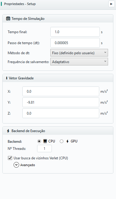
The Settings panel groups the solver time parameters:
| FIELD | UNIT | MEANING |
|---|---|---|
| Final time | s | Final physical simulation time |
| Timestep (dt) | s | Δt - calculated or manually defined |
| dt method | — | Fixed or Rayleigh (automatic) |
| Save frequency | — | Adaptive or fixed snapshot recording interval |
12.2 Timestep method
Two approaches are available:
- Fixed - value entered by the user; this is the initial default and offers reproducible control;
- Rayleigh (automatic) - calculates equation 3.36 from Rayleigh's shortest time between particle materials.
The collision time is not a selectable mode: it can be used as an additional diagnosis. For stiff contacts, small particles, high speeds or cohesion, perform a convergence study by reducing Δt and checking if the quantities of interest remain stable.
12.3 Gravity Vector
Gravity is defined as a vector (X, Y, Z) in m/s2. The default is (0, −9.81, 0). For non-gravity studies (e.g. microgravity mixture or injection tests), just zero the components.
12.4 Execution backend: CPU and GPU
BrixDEM allows you to choose execution backend between CPU and GPU, along with the number of threads (for CPU, via OpenMP) and option Use Verlet Neighbor Search (CPU).
On the GPU backend, Mixed precision computes contacts in FP32. In measured cases, simulation was about 2.5× faster, with a small loss of precision. Enabling it also enables the Verlet neighbor list automatically. The gain depends on the GPU and the case. Turn it off when calibrating materials, comparing against CPU, or completing a sensitivity study; keep the time step and initial conditions the same.
Verlet Neighbor Search and the margin (skin)
To calculate contacts, solver needs to know which particles are close to each particle. Recalculating this list of neighbors from scratch every step is expensive. A Verlet search builds a list of neighbors with clearance - including particles that are up to an extra distance, margin (skin), in addition to the contact radius - and reuses it for several steps, instead of always rebuilding it.
The logic is: as long as no particle has moved more than half the margin, any new contact is already within the list with slack. The list is only rebuilt when the maximum cumulative displacement reaches half the margin. This trades some memory and candidate checks for a substantial reduction in contact-search work.
| CONFIGURATION | EFFECT | HOW TO HELP |
|---|---|---|
| Small margin (skin) | Rebuilds the list frequently; each list is lean | Good for fast/disperse flows |
| Large (skin) margin | Rebuilds rarely, but examines more candidates per step | Good for slow/dense flows |
| Default value (~1⁄2 of maximum radius) | Recommended balance | Keep unless a specific need requires adjustment |
12.5 Snapshot recording frequency
The recording frequency controls how many snapshots the solver records throughout the simulation (see Chapter 15.2). There are two ways:
- Adaptive - particle files follow the same cadence as the visual stream (about 300 frames per simulation). Each visual frame has a particle file at the same step; the interface uses that file to materialize scalars and calculate residence time. The interval is rounded up from the total number of steps divided by 300; step zero and the final frame may also be written, so the count is usually around 300–301. Doubling the final time increases the interval in the same proportion and keeps approximately the same number of frames;
- Fixed interval - you directly specify how many steps elapse between recordings (each N steps).
Example: Final time 0.35 s with Δt = 5×10⁻⁶ s takes 70 000 steps; setting a fixed interval of 700 steps produces about 100 snapshots. Saving very often generates many files and occupies disk; saving infrequently loses temporal detail in fast events (impacts, stack formation). A target of 100–300 snapshots is usually a good balance.
12.6 Timestep with breakage
Smaller fragments reduce Rayleigh time and may require a much smaller step than fed particles. The GUI already provides a suggestion in the Ab-t10 dialog's Timestep (dt) card: Normal uses fed particles, Suggested includes an estimate of the smallest fragments, and Current is the project's selected step. Editing parameters updates the estimate; the card does not change the project timestep automatically.
- In Setup, start with a Rayleigh factor of 0.05–0.1 for breakage; 0.2 may be aggressive. The suggestion uses the configured factor and also considers free-body limits, so it does not assume that 0.05–0.1 has already been selected.
- Check Normal, Suggested and Current after changing material, PSD, CGF or fragmentation resolution. Click Use suggested dt to switch the project to a fixed step at the displayed value. This button does not save other breakage parameters: confirm those with Apply.
- Check the step in Setup and run a short case. The d_min cutoff prevents rebreakage but does not prevent smaller fragments from being born; the suggestion is an estimate, not a stability guarantee.
If fracture occurs at excessive overlap, stop to investigate timestep, configuration and calibration. Reducing Young’s modulus also changes absorbed energy: retain consistency with DWT calibration and wall material as explained in 10.7 and 10.10.